二値分類問題
Kerasライブラリに組み込まれている二値分類のチュートリアル
IMDbデータセットは50000件の映画レビューを「肯定的」「否定的」なデータに分類する問題
データセットは訓練用とテスト用に25000件ずつ、肯定、否定ともに50%ずつのデータで構成されているらしい
データセットはなぜ訓練用とテスト用に分かれているのか
訓練データとテストデータが同じだと、まだ見たことないデータに対して、そのモデルがどれだけの正解率を導き出せるかわからないから。
機械学習では過学習(Over fitting)という問題がある。
これはモデルが訓練データに特化しすぎてしまうこと。
訓練で経験済みのデータに対する正解率は高くなるが、見たことないデータに対する正解率は悪くなってしまう。
そこで過学習になっていないか見極めるために訓練データとテストデータを分けて検証することが大切だということ。
前置き終わり。
サンプルデータを読み込む
from keras.datasets import imdb

# 出現頻度が最も高い10,000個の単語を取得
(train_data, train_labels), (test_data, test_labels) = imdb.load_data(num_words=10000)
訓練データの中身
とりあえず訓練データの中身がどうなっているか確認してみる
# 単語のインデックスに単語をマッピングするクラス
word_index = imdb.get_word_index()
train_data[0]
>> [1, 14, 22, 16, 43, 530, 973,...178, 32]
単語をマッピング
# 辞書データを取得
reverse_word_index = dict([(value, key) for (key, value) in word_index.items()])
# 訓練データの1件目のデータを辞書データに参照して単語を取り出す
# 0;パディング, 1:シーケンス開始, 2:不明の予約語になっているため
decoded_review = ' '.join([reverse_word_index.get(i - 3, '?') for i in train_data[0]])

# 単語を出力
decoded_review

>> "? this film was just brilliant casting location scenery story direction everyone's really suited the part they played and you could just imagine being there robert ? is an amazing actor and now the same being director ? father came from the same scottish island as myself so i loved the fact there was a real connection with this film the witty remarks throughout the film were great it was just brilliant so much that i bought the film as soon as it was released for ? and would recommend it to everyone to watch and the fly fishing was amazing really cried at the end it was so sad and you know what they say if you cry at a film it must have been good and this definitely was also ? to the two little boy's that played the ? of norman and paul they were just brilliant children are often left out of the ? list i think because the stars that play them all grown up are such a big profile for the whole film but these children are amazing and should be praised for what they have done don't you think the whole story was so lovely because it was true and was someone's life after all that was shared with us all"
機械学習開始
データの中身を確認できたところで二値問題に取り組みたいと思います。
まずは訓練データとテストデータを機械学習用に変換します。
データ構造が10000 * 10000の二値問題なので二次元テンソル(samples, features)モデルを使います。
ということでOne-Hot型に変換します
One-Hotエンコーディング関数定義
# one-hot encodeing
import numpy as np

def convertToOneHot(sequences, dimension=1000):
    """
    行列データをOne-Hotエンコーディングする関数
    Parameters
    ----------
    sequences : 行列データ
        行列データ※one-hotエンコーディング対象データ
    dimension : 要素数
    """
    # 0埋めの行列を作成
    results = np.zeros((len(sequences), dimension))
    for i, sequence in enumerate(sequences):
        # i行目 sequence列に1を立てる
        results[i, sequence] = 1.
        return results
訓練データをベクトルデータへ変換
One-Hotエンコーディング関数を使ってベクトルデータへ変換
# 訓練データをベクトル化
x_train = convertToOneHot(train_data, 10000)
# テストデータをベクトル化
x_test = convertToOneHot(test_data, 10000)

x_train[0]
>> array([0., 1., 1., ..., 0., 0., 0.])
ラベルデータもモデル用に変換
ラベルをベクトル化
# ラベルをベクトル化 二値分類(0 ,1)なのでラベルはスカラー値(0と1)が入っている
y_train = np.asarray(train_labels).astype('float32')
y_test  = np.asarray(test_labels).astype('float32')
ニューラルネットワークの構築とモデルの定義
モデルを設計します
レイヤー層のタイプ、出入力数、活性化関数のタイプ、そして層の数を設計します
from keras import models
from keras import layers

model = models.Sequential()
model.add(layers.Dense(16, activation='relu', input_shape=(10000,)))
model.add(layers.Dense(16, activation='relu'))
model.add(layers.Dense(1, activation='sigmoid'))
訓練の妥当性の検証のためのデータを小分けします
x_val = x_train[:10000]
partial_x_train = x_train[10000:]

y_val = y_train[:10000]
partial_y_train = y_train[10000:]
モデルの実装
from keras import optimizers
from keras import losses
from keras import metrics

# モデルを実装
>> model.compile(
    optimizer=optimizers.RMSprop(lr=0.001), # 'rmsprop'
    loss=losses.binary_crossentropy, # 'binary_crossentropy'
    metrics=['acc'] # 'accuracy'
)

# 訓練の実施
history = model.fit(
    partial_x_train,
    partial_y_train,
    epochs=20,
    batch_size=512,
    validation_data=(x_val, y_val)
)
訓練データの確認
model.fit()関数は各エポック毎にHistoryオブジェクトを返す
Historyオブジェクトは訓練データと検証データの損失値と正解率をそれぞれ返します
history_dict = history.history
history_dict.keys()
>> dict_keys(['val_acc', 'acc', 'val_loss', 'loss'])
訓練データと検証データの損失値をプロット
import matplotlib.pyplot as plt
history_dict = history.history
loss_values = history_dict['loss']
val_loss_values = history_dict['val_loss']
epochs = range(1, len(loss_values) + 1)
# bo = bulue dot
plt.plot(epochs, loss_values, 'bo', label='Training loss') # 青のドット 訓練データ
# b = solid bulue line
plt.plot(epochs, val_loss_values, 'b', label='Validation loss') # 青の実践 検証データ
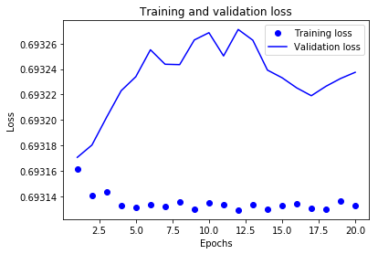
plt.title('Training and validation loss')
plt.xlabel('Epochs')
plt.ylabel('Loss')
plt.legend()
plt.show()
モデルの検証
ドットは訓練データ、実践は検証データ
訓練データの損失値はエポックを重ねるごとに小さくなっているが検証データでは上昇している。
これは過学習であることを示している。
この例でいうと、8-9エポック辺りが損失値が最小になっているため、今回の設計したニューラルネットワーク層の場合はエポック数はそのあたりにしておくのが良いのかもしれない。
そもそも、ニューラルネットワークのレイヤーの設計を見直す必要があるかもしれない。
と、いったことがこのようにグラフを出力することで検証できるということ。
上記では損失率を出力しているが、lossの箇所をaccとすれば正解率をプロットできる。
再訓練
今回はエポック数だけ変えてみたが必要に応じて、活性化関数やレイヤー数、出力数などを変えてみる。
# モデルの訓練をやり直す
model = models.Sequential()
model.add(layers.Dense(16, activation='relu', input_shape=(10000,)))
model.add(layers.Dense(16, activation='relu'))
model.add(layers.Dense(1, activation='sigmoid'))

model.compile(optimizer='rmsprop', loss='binary_crossentropy', metrics=['accuracy'])
model.fit(x_train, y_train, epochs=8, batch_size=512)
# バッチごとにある入力データにおける損失値を計算
results = model.evaluate(x_test, y_test)

>> [0.693177899570465, 0.5]
実データで検証
# 入力サンプルに対する予測値の出力を生成する関数
model.predict(x_test)

>> array([[0.48566884],
       [0.49602675],
       [0.49602675],
       ...,
       [0.49602675],
       [0.49602675],
       [0.49602675]], dtype=float32)
正答率がよくない。
どこかを見直せということでしょう。
振り返り
[学んだこと]
- 二値分類を扱う場合 ラベルは0か1
- 訓練(テスト)データをOne-Hot型に変換
- 隠れ層の活性化関数はReLUを使った
- 隠れ層はDense層を使った
- 出力層の活性化関数はシグモイド関数を使った
- 損失関数はbinary_crossentropyを使った
- オプティマイザはrmspropを使った
- 訓練データにモデルが慣れ、正解率があがるとどこかで過学習に陥り、訓練データ以外のデータでは性能が落ちる
[なんでかなー]
とりあえず、使い方はわかってきたが、正答率が低いということはモデルの設計が悪い、訓練のさせ方が悪いなどが原因なのだろうか。
課題
- 隠れ層の数を変えてみる
- 隠れ層のユニット数を変更してみる
- 損失関数をmseに変更してみる