離散フーリエ変換を再帰で効率よく行う (高速フーリエ変換)

離散フーリエ変換とは

この記事では、波形を表す $N$ 要素の複素数の配列

$$
f = [f(0), f(1), \ldots , f(N-1)]
$$

から、この波形の周波数成分を表す $N$ 要素の複素数の配列

$$
F = [F(0), F(1), \ldots , F(N-1)]
$$

を求めることを、離散フーリエ変換と呼ぶ。
このとき、これらの配列の要素の値には

$$
F(k) = \sum_{n=0}^{N-1} f(n)e^{-i \frac{2 \pi}{N} k n}
$$

という関係が成り立つ。
(他の定義を用いる場合もあるが、この記事ではこの関係が成り立つとする)

また、以下の関係式を用いて、周波数成分を表す配列から波形を表す配列を求めることもできる。

$$
f(n) = \frac{1}{N} \sum_{k=0}^{N-1} F(k)e^{i \frac{2 \pi}{N} k n}
$$

これを離散逆フーリエ変換と呼ぶ。

ここで、実数 $\theta$ について

$$
e^{i \theta} = \cos \theta + i \sin \theta
$$

である。

これらの関係を用いて愚直に離散フーリエ変換を行うと、$N$ 要素ある配列 $F$ のそれぞれの要素の値 $F(k)$ を求めるために、それぞれ $N$ 個の値の合計を求めることになるので、$O(N^2)$ の計算量になる。
この計算量では、だいたい要素数 2,048 程度の計算に 1 秒程度かかることが予想され、たとえば音声信号の波形の周波数成分をリアルタイムで表示したい場合には遅いといえるだろう。
そこで、計算方法を工夫し、離散フーリエ変換の結果を効率よく求めることができるようにしたい。

ω を用いて表す

$$
\omega = e^{-i \frac{2 \pi}{N}}
$$

とおくと、離散フーリエ変換の関係式は

$$
F(k) = \sum_{n=0}^{N-1} f(n) \omega^{ k n}
$$

離散逆フーリエ変換の関係式は

$$
f(n) = \frac{1}{N} \sum_{k=0}^{N-1} F(k)\left(\omega^{-1}\right)^{k n}
$$

と表せる。また、

$$
e^{2 \pi i} = \cos 2\pi + i \sin 2\pi = 1
$$

なので、任意の整数 $m$ について

$$
\omega^{mN} = 1
$$

となる。

たとえば、$N = 8$ のときを考えると

$$
\begin{eqnarray}
F(0) &=& f(0) \omega^0 + f(1) \omega^0 + f(2) \omega^0 + f(3) \omega^0 + f(4) \omega^0 + f(5) \omega^0 + f(6) \omega^0 + f(7) \omega^0 \\
F(1) &=& f(0) \omega^0 + f(1) \omega^1 + f(2) \omega^2 + f(3) \omega^3 + f(4) \omega^4 + f(5) \omega^5 + f(6) \omega^6 + f(7) \omega^7 \\
F(2) &=& f(0) \omega^0 + f(1) \omega^2 + f(2) \omega^4 + f(3) \omega^6 + f(4) \omega^8 + f(5) \omega^{10} + f(6) \omega^{12} + f(7) \omega^{14} \\
F(3) &=& f(0) \omega^0 + f(1) \omega^3 + f(2) \omega^6 + f(3) \omega^9 + f(4) \omega^{12} + f(5) \omega^{15} + f(6) \omega^{18} + f(7) \omega^{21} \\
F(4) &=& f(0) \omega^0 + f(1) \omega^4 + f(2) \omega^8 + f(3) \omega^{12} + f(4) \omega^{16} + f(5) \omega^{20} + f(6) \omega^{24} + f(7) \omega^{28} \\
F(5) &=& f(0) \omega^0 + f(1) \omega^5 + f(2) \omega^{10} + f(3) \omega^{15} + f(4) \omega^{20} + f(5) \omega^{25} + f(6) \omega^{30} + f(7) \omega^{35} \\
F(6) &=& f(0) \omega^0 + f(1) \omega^6 + f(2) \omega^{12} + f(3) \omega^{18} + f(4) \omega^{24} + f(5) \omega^{30} + f(6) \omega^{36} + f(7) \omega^{42} \\
F(7) &=& f(0) \omega^0 + f(1) \omega^7 + f(2) \omega^{14} + f(3) \omega^{21} + f(4) \omega^{28} + f(5) \omega^{35} + f(6) \omega^{42} + f(7) \omega^{49}
\end{eqnarray}
$$

すなわち

$$
\left(
\begin{array}{l}
F(0) \\ F(1) \\ F(2) \\ F(3) \\ F(4) \\ F(5) \\ F(6) \\ F(7) \\
\end{array}
\right) = \left(
\begin{array}{llllllll}
\omega^0 & \omega^0 & \omega^0 & \omega^0 & \omega^0 & \omega^0 & \omega^0 & \omega^0 \\
\omega^0 & \omega^1 & \omega^2 & \omega^3 & \omega^4 & \omega^5 & \omega^6 & \omega^7 \\
\omega^0 & \omega^2 & \omega^4 & \omega^6 & \omega^8 & \omega^{10} & \omega^{12} & \omega^{14} \\
\omega^0 & \omega^3 & \omega^6 & \omega^9 & \omega^{12} & \omega^{15} & \omega^{18} & \omega^{21} \\
\omega^0 & \omega^4 & \omega^8 & \omega^{12} & \omega^{16} & \omega^{20} & \omega^{24} & \omega^{28} \\
\omega^0 & \omega^5 & \omega^{10} & \omega^{15} & \omega^{20} & \omega^{25} & \omega^{30} & \omega^{35} \\
\omega^0 & \omega^6 & \omega^{12} & \omega^{18} & \omega^{24} & \omega^{30} & \omega^{36} & \omega^{42} \\
\omega^0 & \omega^7 & \omega^{14} & \omega^{21} & \omega^{28} & \omega^{35} & \omega^{42} & \omega^{49}
\end{array}
\right) \left(
\begin{array}{l}
f(0) \\ f(1) \\ f(2) \\ f(3) \\ f(4) \\ f(5) \\ f(6) \\ f(7) \\
\end{array}
\right)
$$

と表せる。

添字の偶奇でグループ分けし、変形する

$N = 8$ の場合の離散フーリエ変換の関係式を展開したものを、出力の添字が偶数の要素・奇数の要素がそれぞれまとまるように並べ替えてみる。

$$
\left(
\begin{array}{l}
F(0) \\ F(2) \\ F(4) \\ F(6) \\ F(1) \\ F(3) \\ F(5) \\ F(7) \\
\end{array}
\right) = \left(
\begin{array}{llllllll}
\omega^0 & \omega^0 & \omega^0 & \omega^0 & \omega^0 & \omega^0 & \omega^0 & \omega^0 \\
\omega^0 & \omega^2 & \omega^4 & \omega^6 & \omega^8 & \omega^{10} & \omega^{12} & \omega^{14} \\
\omega^0 & \omega^4 & \omega^8 & \omega^{12} & \omega^{16} & \omega^{20} & \omega^{24} & \omega^{28} \\
\omega^0 & \omega^6 & \omega^{12} & \omega^{18} & \omega^{24} & \omega^{30} & \omega^{36} & \omega^{42} \\
\omega^0 & \omega^1 & \omega^2 & \omega^3 & \omega^4 & \omega^5 & \omega^6 & \omega^7 \\
\omega^0 & \omega^3 & \omega^6 & \omega^9 & \omega^{12} & \omega^{15} & \omega^{18} & \omega^{21} \\
\omega^0 & \omega^5 & \omega^{10} & \omega^{15} & \omega^{20} & \omega^{25} & \omega^{30} & \omega^{35} \\
\omega^0 & \omega^7 & \omega^{14} & \omega^{21} & \omega^{28} & \omega^{35} & \omega^{42} & \omega^{49}
\end{array}
\right) \left(
\begin{array}{l}
f(0) \\ f(1) \\ f(2) \\ f(3) \\ f(4) \\ f(5) \\ f(6) \\ f(7) \\
\end{array}
\right)
$$

さらに、8×8 の係数行列を 4×4 ずつに分割する。

$$
\begin{eqnarray}
\left(
\begin{array}{l}
F(0) \\ F(2) \\ F(4) \\ F(6)
\end{array}
\right) &=& \left(
\begin{array}{llll}
\omega^0 & \omega^0 & \omega^0 & \omega^0 \\
\omega^0 & \omega^2 & \omega^4 & \omega^6 \\
\omega^0 & \omega^4 & \omega^8 & \omega^{12} \\
\omega^0 & \omega^6 & \omega^{12} & \omega^{18}
\end{array}
\right) \left(
\begin{array}{l}
f(0) \\ f(1) \\ f(2) \\ f(3)
\end{array}
\right) + \left(
\begin{array}{llll}
\omega^0 & \omega^0 & \omega^0 & \omega^0 \\
\omega^8 & \omega^{10} & \omega^{12} & \omega^{14} \\
\omega^{16} & \omega^{20} & \omega^{24} & \omega^{28} \\
\omega^{24} & \omega^{30} & \omega^{36} & \omega^{42}
\end{array}
\right) \left(
\begin{array}{l}
f(4) \\ f(5) \\ f(6) \\ f(7) \\
\end{array}
\right)
\\
\left(
\begin{array}{l}
F(1) \\ F(3) \\ F(5) \\ F(7)
\end{array}
\right) &=& \left(
\begin{array}{llll}
\omega^0 & \omega^1 & \omega^2 & \omega^3 \\
\omega^0 & \omega^3 & \omega^6 & \omega^9 \\
\omega^0 & \omega^5 & \omega^{10} & \omega^{15} \\
\omega^0 & \omega^7 & \omega^{14} & \omega^{21}
\end{array}
\right) \left(
\begin{array}{l}
f(0) \\ f(1) \\ f(2) \\ f(3)
\end{array}
\right) + \left(
\begin{array}{llll}
\omega^4 & \omega^5 & \omega^6 & \omega^7 \\
\omega^{12} & \omega^{15} & \omega^{18} & \omega^{21} \\
\omega^{20} & \omega^{25} & \omega^{30} & \omega^{35} \\
\omega^{28} & \omega^{35} & \omega^{42} & \omega^{49}
\end{array}
\right) \left(
\begin{array}{l}
f(4) \\ f(5) \\ f(6) \\ f(7) \\
\end{array}
\right)
\end{eqnarray}
$$

$N = 8$ のとき、$\omega^4 = -1, \omega^8 = 1$ なので、

$$
\begin{eqnarray}
\omega^0 = \omega^8 = \omega^{16} = \omega^{24} &=& 1 \\
\omega^4 = \omega^{12} = \omega^{20} = \omega^{28} &=& -1
\end{eqnarray}
$$

がいえる。これを用いて変形すると

$$
\begin{eqnarray}
\left(
\begin{array}{l}
F(0) \\ F(2) \\ F(4) \\ F(6)
\end{array}
\right) &=& \left(
\begin{array}{llll}
\omega^0 & \omega^0 & \omega^0 & \omega^0 \\
\omega^0 & \omega^2 & \omega^4 & \omega^6 \\
\omega^0 & \omega^4 & \omega^8 & \omega^{12} \\
\omega^0 & \omega^6 & \omega^{12} & \omega^{18}
\end{array}
\right) \left(
\begin{array}{l}
f(0) \\ f(1) \\ f(2) \\ f(3)
\end{array}
\right) + \left(
\begin{array}{llll}
\omega^0 & \omega^0 & \omega^0 & \omega^0 \\
\omega^0 & \omega^2 & \omega^4 & \omega^6 \\
\omega^0 & \omega^4 & \omega^8 & \omega^{12} \\
\omega^0 & \omega^6 & \omega^{12} & \omega^{18}
\end{array}
\right) \left(
\begin{array}{l}
f(4) \\ f(5) \\ f(6) \\ f(7) \\
\end{array}
\right)
\\
\left(
\begin{array}{l}
F(1) \\ F(3) \\ F(5) \\ F(7)
\end{array}
\right) &=& \left(
\begin{array}{llll}
\omega^0 & \omega^1 & \omega^2 & \omega^3 \\
\omega^0 & \omega^3 & \omega^6 & \omega^9 \\
\omega^0 & \omega^5 & \omega^{10} & \omega^{15} \\
\omega^0 & \omega^7 & \omega^{14} & \omega^{21}
\end{array}
\right) \left(
\begin{array}{l}
f(0) \\ f(1) \\ f(2) \\ f(3)
\end{array}
\right) - \left(
\begin{array}{llll}
\omega^0 & \omega^1 & \omega^2 & \omega^3 \\
\omega^0 & \omega^3 & \omega^6 & \omega^9 \\
\omega^0 & \omega^5 & \omega^{10} & \omega^{15} \\
\omega^0 & \omega^7 & \omega^{14} & \omega^{21}
\end{array}
\right) \left(
\begin{array}{l}
f(4) \\ f(5) \\ f(6) \\ f(7) \\
\end{array}
\right)
\end{eqnarray}
$$

すなわち

$$
\begin{eqnarray}
\left(
\begin{array}{l}
F(0) \\ F(2) \\ F(4) \\ F(6)
\end{array}
\right) &=& \left(
\begin{array}{llll}
\omega^0 & \omega^0 & \omega^0 & \omega^0 \\
\omega^0 & \omega^2 & \omega^4 & \omega^6 \\
\omega^0 & \omega^4 & \omega^8 & \omega^{12} \\
\omega^0 & \omega^6 & \omega^{12} & \omega^{18}
\end{array}
\right) \left(
\begin{array}{l}
f(0) + f(4) \\ f(1) + f(5) \\ f(2) + f(6) \\ f(3) + f(7)
\end{array}
\right)
\\
\left(
\begin{array}{l}
F(1) \\ F(3) \\ F(5) \\ F(7)
\end{array}
\right) &=& \left(
\begin{array}{llll}
\omega^0 & \omega^1 & \omega^2 & \omega^3 \\
\omega^0 & \omega^3 & \omega^6 & \omega^9 \\
\omega^0 & \omega^5 & \omega^{10} & \omega^{15} \\
\omega^0 & \omega^7 & \omega^{14} & \omega^{21}
\end{array}
\right) \left(
\begin{array}{l}
f(0) - f(4) \\ f(1) - f(5) \ \\ f(2) - f(6) \\ f(3) - f(7)
\end{array}
\right)
\end{eqnarray}
$$

となる。
さらに、2番目の係数行列を1番目の係数行列に合わせるため、$\omega^0, \omega^1, \omega^2, \omega^3$ の掛け算をそれぞれベクトル側に移すと、以下のようになる。

$$
\left(
\begin{array}{l}
F(1) \\ F(3) \\ F(5) \\ F(7)
\end{array}
\right) = \left(
\begin{array}{llll}
\omega^0 & \omega^0 & \omega^0 & \omega^0 \\
\omega^0 & \omega^2 & \omega^4 & \omega^6 \\
\omega^0 & \omega^4 & \omega^8 & \omega^{12} \\
\omega^0 & \omega^6 & \omega^{12} & \omega^{18}
\end{array}
\right) \left(
\begin{array}{l}
\omega^0 \left( f(0) - f(4) \right) \\
\omega^1 \left( f(1) - f(5) \right) \\
\omega^2 \left( f(2) - f(6) \right) \\
\omega^3 \left( f(3) - f(7) \right)
\end{array}
\right)
$$

ここで、$\omega_* = \omega^2$ とおくと、これらの関係式は

$$
\begin{eqnarray}
\left(
\begin{array}{l}
F(0) \\ F(2) \\ F(4) \\ F(6)
\end{array}
\right) &=& \left(
\begin{array}{llll}
\omega_*^0 & \omega_*^0 & \omega_*^0 & \omega_*^0 \\
\omega_*^0 & \omega_*^1 & \omega_*^2 & \omega_*^3 \\
\omega_*^0 & \omega_*^2 & \omega_*^4 & \omega_*^6 \\
\omega_*^0 & \omega_*^3 & \omega_*^6 & \omega_*^9
\end{array}
\right) \left(
\begin{array}{l}
f(0) + f(4) \\ f(1) + f(5) \\ f(2) + f(6) \\ f(3) + f(7)
\end{array}
\right)
\\
\left(
\begin{array}{l}
F(1) \\ F(3) \\ F(5) \\ F(7)
\end{array}
\right) &=& \left(
\begin{array}{llll}
\omega_*^0 & \omega_*^0 & \omega_*^0 & \omega_*^0 \\
\omega_*^0 & \omega_*^1 & \omega_*^2 & \omega_*^3 \\
\omega_*^0 & \omega_*^2 & \omega_*^4 & \omega_*^6 \\
\omega_*^0 & \omega_*^3 & \omega_*^6 & \omega_*^9
\end{array}
\right) \left(
\begin{array}{l}
\omega^0 \left( f(0) - f(4) \right) \\
\omega^1 \left( f(1) - f(5) \right) \\
\omega^2 \left( f(2) - f(6) \right) \\
\omega^3 \left( f(3) - f(7) \right)
\end{array}
\right)
\end{eqnarray}
$$

となる。

$$
\omega_* = \omega^2 = {\left(e^{-i \frac{2 \pi}{N}}\right)}^2 = e^{-i \frac{2 \pi}{N/2}}
$$

なので、これは、$N$ が偶数のとき、$N$ 要素の配列の離散フーリエ変換の結果は $N/2$ 要素の配列の離散フーリエ変換を用いて求めることができることを示している。

計算量が減ることを確認する

$N$ 要素の配列の離散フーリエ変換を愚直に行う場合と $N/2$ 要素の配列の離散フーリエ変換を用いて行う場合で計算量を比較し、後者のほうが計算量が減ることを確認する。
ただし、$\omega^k$ の値は離散フーリエ変換の入力に依存せず、事前に求めてテーブルに格納しておくことができるので、 $\omega^k$ の値を求めるための計算量はここでは考えない。

$N$ 要素の配列の離散フーリエ変換を愚直に行う場合、結果の1要素を求めるのに $N$ 回の乗算と $N-1$ 回の加算を行うので、$N$ 要素の結果全体を求めるには $N^2 (N-1)$ 回の演算をすることになる。

一方、$N$ 要素の配列の離散フーリエ変換を $N/2$ 要素の配列の離散フーリエ変換を用いて求める場合、$N/2$ 要素の配列の離散フーリエ変換を2回行うため $2 {(N/2)}^2 (N/2-1)$ 回の演算をすることになる。
さらに、これらの $N/2$ 要素の配列の離散フーリエ変換の入力を求めるために $N$ 回の加算、$N$ 回の減算、$N-1$ 回の乗算を行う。($\omega^0 = 1$ なので、$\omega^0$ の乗算は省略できる)
よって、合わせて $2 {(N/2)}^2 (N/2-1) + 3N - 1$ 回の演算をすることになる。

$N/2$ 要素の配列の離散フーリエ変換に用いる $\omega_*^k$ の値は、$\omega^k$ の値のテーブルを1要素おきに参照すればわかり、新たに求める必要は無い。

これらの演算回数を引き算することで、比較する。

$$
\begin{eqnarray}
&& N^2 (N-1) - \left( 2{\left(\frac{N}{2}\right)}^2 \left(\frac{N}{2} - 1 \right) + 3N - 1 \right) \\
&=& N^3 - N^2 - \frac{1}{4} N^3 + \frac{1}{2} N^2 - 3N + 1 \\
&=& \frac{3}{4} N^3 - \frac{1}{2} N^2 - 3N + 1
\end{eqnarray}
$$

プロットしてみると、$N = 2$ では離散フーリエ変換を愚直に行った方が演算回数が少なくなるが、$N \geq 4$ では $N/2$ 要素の配列の離散フーリエ変換を用いたほうが演算回数が少なくなることがわかる。

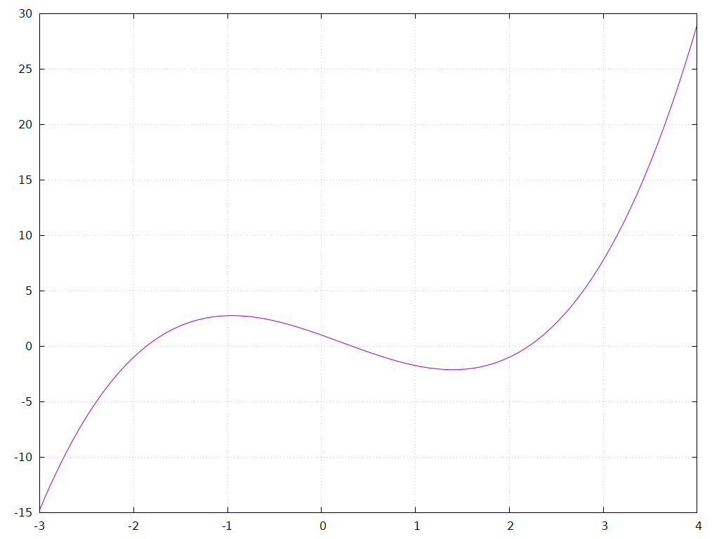
ただし、実際に計算を行う場合、関数呼び出しのオーバーヘッドなどの影響で、効率が逆転する $N$ はもう少し大きいかもしれない。

さらに、$N/2$ 要素の離散フーリエ変換を $N/4$ 要素の離散フーリエ変換を用いて求め、$N/4$ 要素の離散フーリエ変換を $N/8$ 要素の離散フーリエ変換を用いて求め…のように、要素数が偶数である限り再帰的に計算を行うことで、さらに効率を上げることができるだろう。
入力の要素数 $N$ を 2 のべき乗にしておくと、この効率化を最大限活用できる。

実装

C言語 (C99) で実装を行った。

愚直な実装

$N/2$ 要素の離散フーリエ変換を用いずに、$N$ 要素の離散フーリエ変換をそのまま行う。

dft.c

#include <stddef.h>
#include <complex.h>

#define PI 3.141592653589793238462643383279

void dft(double complex *out, const double complex *in, size_t size) {
	for (size_t k = 0; k < size; k++) {
		out[k] = 0;
		for (size_t n = 0; n < size; n++) {
			out[k] += in[n] * cexp(-2 * I * PI * k * n / size);
		}
	}
}

素直な実装

$N$ が偶数ならば、$N/2$ 要素の離散フーリエ変換を利用して $N$ 要素の離散フーリエ変換を求める。
$N$ が奇数のときは、$N$ 要素の離散フーリエ変換をそのまま行う。
最初の $N$ が正の整数であれば、2 で割ることを繰り返せばいつかは必ず奇数になるので、このアルゴリズムで再帰は必ず停止し、計算が可能である。

fft.c

#include <stdlib.h>
#include <complex.h>
#include <assert.h>

#define PI 3.141592653589793238462643383279

void fft(double complex *out, const double complex *in, size_t size) {
	if (size % 2 != 0) {
		for (size_t k = 0; k < size; k++) {
			out[k] = 0;
			for (size_t n = 0; n < size; n++) {
				out[k] += in[n] * cexp(-2 * I * PI * k * n / size);
			}
		}
	} else {
		double complex *out1, *out2, *in1, *in2;
		assert(size / 2 > 0);
		out1 = malloc(sizeof(*out1) * (size / 2));
		out2 = malloc(sizeof(*out2) * (size / 2));
		in1 = malloc(sizeof(*in1) * (size / 2));
		in2 = malloc(sizeof(*in2) * (size / 2));
		if (out1 == NULL || out2 == NULL || in1 == NULL || in2 == NULL) exit(2);
		for (size_t i = 0; i < size / 2; i++) {
			in1[i] = in[i] + in[i + size / 2];
			in2[i] = cexp(-2 * I * PI * i / size) * (in[i] - in[i + size / 2]);
		}
		fft(out1, in1, size / 2);
		fft(out2, in2, size / 2);
		for (size_t i = 0; i < size / 2; i++) {
			out[i * 2] = out1[i];
			out[i * 2 + 1] = out2[i];
		}
		free(out1);
		free(out2);
		free(in1);
		free(in2);
	}
}

assert を入れない場合、今回の検証において、in1 および in2 が初期化せずに使用される可能性があるという警告が出力された。

工夫した実装

$N/2$ 要素の離散フーリエ変換を用いて $N$ 要素の離散フーリエ変換を求める際に配列の使い回しを行い、メモリの確保・解放やデータのコピーを削減した。
具体的には、入力については後段に渡す値を計算したらもとの値はもう使用しないので、後段の後段にわたす値を格納する領域として再利用するようにした。
さらに、出力については格納する位置と間隔を後段に渡すことで、結果をコピーせずに直接格納できるようにした。

fft2.c

#include <stdlib.h>
#include <string.h>
#include <complex.h>

#define PI 3.141592653589793238462643383279

static void fft2_internal(double complex *out, double complex *buf, double complex *in, size_t size, size_t out_stride) {
	if (size % 2 != 0) {
		for (size_t k = 0; k < size; k++) {
			out[k * out_stride] = 0;
			for (size_t n = 0; n < size; n++) {
				out[k * out_stride] += in[n] * cexp(-2 * I * PI * k * n / size);
			}
		}
	} else {
		for (size_t i = 0; i < size / 2; i++) {
			buf[i] = in[i] + in[i + size / 2];
			buf[i + size / 2] = cexp(-2 * I * PI * i / size) * (in[i] - in[i + size / 2]);
		}
		fft2_internal(out, in, buf, size / 2, out_stride * 2);
		fft2_internal(out + out_stride, in + size / 2, buf + size / 2, size / 2, out_stride * 2);
	}
}

void fft2(double complex *out, double complex *in, size_t size) {
	double complex *buf1, *buf2;
	buf1 = malloc(sizeof(*buf1) * size);
	buf2 = malloc(sizeof(*buf2) * size);
	if (buf1 == NULL || buf2 == NULL) exit(2);
	memcpy(buf2, in, sizeof(*buf2) * size);
	fft2_internal(out, buf1, buf2, size, 1);
	free(buf1);
	free(buf2);
}

さらに工夫した実装

「工夫した実装」に加え、$\omega$ の累乗の表を最初に作り、毎回計算しなくていいようにした。

fft3.c

#include <stdlib.h>
#include <string.h>
#include <complex.h>

#define PI 3.141592653589793238462643383279

static void fft3_internal(double complex *out, double complex *buf, double complex *in, const double complex *omega, size_t size, size_t stride) {
	if (size % 2 != 0) {
		for (size_t k = 0; k < size; k++) {
			out[k * stride] = 0;
			for (size_t n = 0; n < size; n++) {
				out[k * stride] += in[n] * omega[k * n % size * stride];
			}
		}
	} else {
		for (size_t i = 0; i < size / 2; i++) {
			buf[i] = in[i] + in[i + size / 2];
			buf[i + size / 2] = omega[i * stride] * (in[i] - in[i + size / 2]);
		}
		fft3_internal(out, in, buf, omega, size / 2, stride * 2);
		fft3_internal(out + stride, in + size / 2, buf + size / 2, omega, size / 2, stride * 2);
	}
}

void fft3(double complex *out, const double complex *in, size_t size) {
	double complex *buf1, *buf2, *omega;
	buf1 = malloc(sizeof(*buf1) * size);
	buf2 = malloc(sizeof(*buf2) * size);
	omega = malloc(sizeof(*omega) * size);
	if (buf1 == NULL || buf2 == NULL || omega == NULL) exit(2);
	memcpy(buf2, in, sizeof(*buf2) * size);
	for (size_t i = 0; i < size; i++) {
		omega[i] = cexp(-2 * I * PI * i / size);
	}
	fft3_internal(out, buf1, buf2, omega, size, 1);
	free(buf1);
	free(buf2);
	free(omega);
}

性能の比較

AWS EC2 (t2.micro) 上の Ubuntu Server 24.04 (AMI ID: ami-04dd23e62ed049936) 上で実行し、実行時間の比較を行った。
CPU は Intel(R) Xeon(R) CPU E5-2686 v4 @ 2.30GHz、コンパイラは gcc 13.2.0 である。

実行にあたり、入出力を行う以下のコードを用意した。

io.c

#include <stdio.h>
#include <stdlib.h>
#include <complex.h>

#ifndef FUNC
#error pleaae define FUNC to the name of the function to use
#endif

void FUNC(double complex *out, const double complex *in, size_t size);

int main(void) {
	size_t size;
	if (scanf("%zu", &size) != 1) return 1;
	double complex *in, *out;
	in = malloc(sizeof(*in) * size);
	out = malloc(sizeof(*out) * size);
	if (in == NULL || out == NULL) {
		fputs("memory allocation error\n", stderr);
		free(in);
		free(out);
		return 2;
	}
	for (size_t i = 0; i < size; i++) {
		double real, imag;
		if (scanf("%lf%lf", &real, &imag) != 2) return 1;
		in[i] = real + I * imag;
	}
	FUNC(out, in, size);
	for (size_t i = 0; i < size; i++) {
		printf("%g %g\n", creal(out[i]), cimag(out[i]));
	}
	free(in);
	free(out);
	return 0;
}

Makefile

CC=gcc
CFLAGS=-O2 -Wall -Wextra -std=c99 -pedantic

.PHONY: all
all: dft fft fft2 fft3

dft: dft.c io.c
	$(CC) $(CFLAGS) -o $@ $^ -DFUNC=dft -lm

fft: fft.c io.c
	$(CC) $(CFLAGS) -o $@ $^ -DFUNC=fft -lm

fft2: fft2.c io.c
	$(CC) $(CFLAGS) -o $@ $^ -DFUNC=fft2 -lm

fft3: fft3.c io.c
	$(CC) $(CFLAGS) -o $@ $^ -DFUNC=fft3 -lm

さらに、以下のコードでランダムな入力を用意した。

gen.py

import sys
import random

size = int(sys.argv[1])

print(size)
for _ in range(size):
	print("%f %f" % (random.random() * 2 - 1, random.random() * 2 - 1))

そして、以下の形式のコマンドで3回実行し、ユーザー時間の平均を求めた。

time ./dft < in_rnd1024.txt > /dev/null

実行時間 (ms) は、以下のようになった。

入力の要素数	1024	2048	4096	8192	16384	32768	65536
愚直な実装	44	173	685	2741	10858	43671	175780
素直な実装	2	3	7	15	28	60	119
工夫した実装	2	3	7	13	27	56	114
さらに工夫した実装	1	4	6	13	25	51	102

「愚直な実装」では入力の要素数を2倍にすると実行時間は約4倍になっている一方、今回用意したそれ以外の実装では入力の要素数を2倍にすると実行時間は約2倍になっている。
また、特に入力の要素数が多い場合において、今回行った

• データのコピーを行う回数を少なくする
• $\omega$ の累乗を保存して使い回す

という工夫は、実行時間を短くする効果がありそうであることがわかった。

結論

要素数が偶数のとき、離散フーリエ変換は半分の要素数の離散フーリエ変換を用いて効率よく行うことができる。

参考資料

• うさぎでもわかる信号処理・制御工学　第13羽　離散フーリエ変換(DFT) | 工業大学生ももやまのうさぎ塾
• うさぎでもわかる信号処理・制御工学　第14羽　高速フーリエ変換(FFT) | 工業大学生ももやまのうさぎ塾
• 離散フーリエ変換入門
• 6. 離散フーリエ変換 (やる夫で学ぶディジタル信号処理)
• オイラーの公式