The Naïve Bayes algorithm is one of the fundamental things to study when studying statistics of artificial intelligence. Here I'm going to explain naive Bayes.
Probability vs likelihood.
Generally, in machine learning, we know that past incidents (data points) are widely used to predict the future. It is not only mattering what happened in the past but also how probable it will be replicated in the future, known as the likelihood of an event occurring in a random space.
Let us take a simple example:
Suppose I have an unbiased 500 yen coin. When I flipped the coin, I can expect it will be the value side (tail). There is a 50% of possibility that my expectation comes true. (There are two possible outcomes, head and tail. Portability is calculated by (expected outcome/total no. of outcomes)
Now let us move a bit deep by operating two experiments at the same time. This time we are additionally rolling a dice. What is the probability of getting head by coin and getting 3 from dice?
The answer can be calculated as below;
P(Head & 3) = P(Head) * P(3) = 1/2 * 1/6 = 1/12
The term for the above example is called joint probability. Other than joint probability, there are two more two types, conditional probability and marginal probability.
- Joint probability (probability of the coin landing on heads AND the dice landing on 3)
- conditional probability (probability of heads GIVEN THAT the dice lands on 3)
- marginal probability (probability of JUST the coin or JUST the dice)
The Bayes’ Theorem
It declares, for two events A & B, if we know the conditional probability of B given A and B's probability, then it is possible to calculate the probability of B given A.

Let us move to a simple example to explain the Bayes rule.

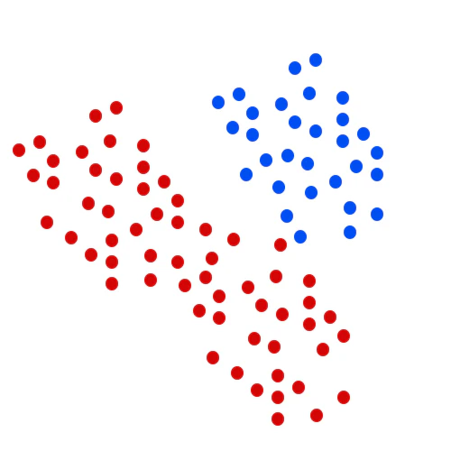
Suppose that I have 30 BLUE objects and 60 RED objects. So there twice as many RED objects as BLUE. If I place a new object, it can be a RED since it is twice likely to happen rather than BLUE. This concept is called prior probability in Bayesian analysis.
Total objects = 90 (BLUE=30 + RED=60)
Prior probability of RED = Number of RED objects / total objects = 60/90
Prior probability of BLUE = Number of BLUE objects / total objects = 30/90
We finished calculating the prior probabilities. Now let us think that the new object is placed. Previously objects are well clustered. So we can assume that the new color of the new object can decide by the number of previous objects around the newly placed one.
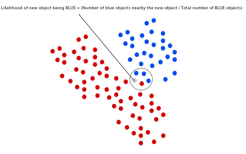
If there are many BLUE objects, it can be BLUE, or If there are many REDS, it can be RED. To measure this likelihood, we form a circle around the new object which contains a number (to be determined a priori) of points regardless of their class names. Then we count the number of points in the circle fitting to each class name.
From hereafter, let us take the new object as X.
From the above drawing, we can see that the likelihood (possibility) of a X given RED is smaller than the likelihood of a X given BLUE since the circle contains the 1 RED and 3 BLUE objects.
In the previous section, the prior probabilities imply that X can relate to the RED since there are twice RED objects than the BLUE objects. However, we can see that likelihood contradicts the above. X can be BLUE since there are more BLUE than the RED around the X. We can calculate the posterior portability by multiplying by prior probability and likelihood.
Posterior Probability of RED=Prior Probability of RED ×Likelihood of RED =60/90×1/60
Posterior Probability of BLUE=Prior Probability of BLUE ×Likelihood of BLUE =30/90×3/30
By analyzing the calculation results, we can classify the new objects that belong to the BLUE since the Posterior Probability of BLUE is larger than the Posterior Probability of RED.
This article will be continued in the next writing...
*本記事は @qualitia_cdevの中の一人、@nuwanさんが書いてくれました。
*This article is written by @nuwan a member of @qualitia_cdev.
