Basic Idea
Variational Information Maximizing Exploration (VIME)[1] improves exploration efficiency by rewarding curiosity. Let's put a parameterized dynamics model of an environment as
$$
s_{t+1} = f(s_t, a_t; \theta) \tag{1}
$$
where $\theta$ is a vector of parameters. Then curiosity is rewarded as follows.
$$
r_t' = r_t + \eta D_{KL}[p(\theta,|,\xi_t,a_t,s_{t+1}),||,p(\theta,|,\xi_t)] \tag{2}
$$
where $\xi_t$ is a history (i.e., all samples). We call the second term curiosity term. The prior $p(\theta,|,\xi_t)$ is a distribution over $\theta$ given the history. The posterior $p(\theta,|,\xi_t,a_t,s_{t+1})$ is an update distribution given an action $a_t$ and its results $s_{t+1}$.
The posterior is practically impossible to compute because the denominator is intractable.
$$
p(\theta,|,\xi_t,a_t,s_{t+1})
= \frac{p(\theta,|,\xi_t),p(s_{t+1},|,\xi_t,a_t;\theta)}{p(s_{t+1},|,\xi_t,a_t)}
= \frac{p(\theta,|,\xi_t),p(s_{t+1},|,\xi_t,a_t;\theta)}{\int_{\Theta} p(s_{t+1},|,\xi_t,a_t;\theta),p(\theta,|,\xi_t),d\theta}
$$
Therefore, it is approximated with a fully factorized Gaussian distribution $q(\theta,;\phi)$.
q(\theta\,;\phi) = \prod^{|\Theta|}_{i=1} \mathcal{N}(\theta_i\,|\,\mu_i, \sigma_i^2) \tag{3}
where $\phi = [\mu^{\rm T}, \rho^{\rm T}]^{\rm T}$ and $\sigma_i = \log(1 + e^{\rho_i})$. Variational inference if conducted to make $q(\theta,;\phi)$ close to the posterior.
\begin{align}
&D_{KL} [q(\theta\,;\phi)\,||\,p(\theta\,|\,D)]\\
&= \int_{\Theta} q(\theta\,;\phi) \left[ \log q(\theta\,;\phi) - p(\theta\,|\,D) \right]\,d\theta\\
&= \int_{\Theta} q(\theta\,;\phi) \left[ \log q(\theta\,;\phi) - \log \frac{p(\theta)\,p(D\,|\,\theta)}{p(D)} \right]\,d\theta\\
&= \int_{\Theta} q(\theta\,;\phi) \left[ \log q(\theta\,;\phi) - \log p(\theta)  - \log p(D\,|\,\theta) + \log p(D) \right]\,d\theta\\
&= \log p(D)
+ \int_{\Theta} q(\theta\,;\phi) \log \frac{q(\theta\,;\phi)}{p(\theta)}\,d\theta  - \int_{\Theta} q(\theta\,;\phi)\log p(D\,|\,\theta)\,d\theta\\
&= \log p(D) - \left( E_{\theta\sim q(\cdot;\phi)}[\log p(D\,|\,\theta)] - D_{KL}[q(\theta\,;\phi)\,||\,p(\theta)] \right) \tag{4}
\end{align}
To minimize $D_{KL} [q(\theta,;\phi),||,p(\theta)]$, you should maximize the second term of (4). This term is evidence lower bound (ELBO). Hence, you will get an approximation of the posterior given samples collected up to t by solving the following optimization.
\begin{align}
\phi_t \leftarrow \mathop{\rm argmax}\limits_{\phi} \left\{ E_{\theta\sim q(\cdot;\phi)}[\log p(D\,|\,\theta)] - D_{KL}[q(\theta\,;\phi)\,||\,p(\theta)] \right\} \tag{5}
\end{align}
Based on this idea, the curiosity reward (1) can be calculated as follows.
$$
r_t' = r_t + \eta D_{KL}[q(\theta,;\phi_{t+1}),||,q(\theta,;\phi_{t})] \tag{6}
$$
Modeling Dynamics with Bayesian Neural Network
The dynamics model $f$ in (1) is implemented as a Bayesian neural network (BNN),
which receives the current observation and action and calculates a mean and variance of the next observation. For computation stability, the natural logarithm of variance within a specific value range is returned. The network parameters $\theta$ (weights and biases) are sampled from a fully factorized Gaussian as in (3).
Local Reparameterization Trick
A naive implementation would be sampling all the network parameters from a multivariate Gaussian parameterized by $\phi = [\mu^{\rm T}, \rho^{\rm T}]^{\rm T}$. However, this is computationally expensive. Thus, a technique called "local parameterization"[2] is used. Instead of directly sampling weights and biases in
a neural network, pre-activation values are sampled.
Suppose a fully connected layer $l$, whose weight and bias are $W$ and $b$, respectively. In a BNN,
\begin{align}
W_{ij} \sim \mathcal{N} (W_{ij}\,|\,\mu _{W _{ij}}, \sigma _{W _{ij}}^2) &\Leftrightarrow W_{ij} = \mu _{W _{ij}} + \sigma _{W _{ij}} \epsilon _{W _{ij}}\\
b _{j} \sim \mathcal{N} (b _{j}\,|\,\mu _{b _{j}}, \sigma _{b _{j}}^2)
&\Leftrightarrow b_{j} = \mu _{b _{j}} + \sigma _{b _{j}} \epsilon _{b _j}
\end{align}
where $\epsilon _{W _{ij}}$ and $\epsilon _{b _{j}}$ are random variable sampled from $\mathcal{N} (\cdot,|,\mathbf{0}, I)$. Pre-activation value $X^{L+1,\prime}$ is calculated as follows.
\begin{align}
X^{L+1\,\prime} &= \sum _{i=1}^{|L|} X _{mi}^{L} W _{ij} + b _{j}\\
&= \sum _{i=1}^{|L|} X _{mi}^{L} (\mu _{W _{ij}} + \sigma _{W _{ij}} \epsilon _{W _{ij}}) + \mu _{b _{j}} + \sigma _{b _{j}} \epsilon _{b _j}
\end{align}
Because of the central limit theorem, $X^{L+1,\prime}$ follows a multivariate Gaussian distribution with the following mean and variance.
\begin{align}
\mathbb{E}[ X^{L+1\,\prime} ] &= \sum _{i=1}^{|L|} X _{mi}^{L} \mu _{W _{ij}} + \mu _{b _{j}}\\
{\rm Var}[ X^{L+1\,\prime} ] &= \sum _{i=1}^{|L|} (X _{mi}^{L})^2 \sigma _{W _{ij}}^2 {\rm Var}[\epsilon _{W _{ij}}] + \sigma _{b _{j}}^2 {\rm Var}[ \epsilon _{b _j} ]\\
&= \sum _{i=1}^{|L|} (X _{mi}^{L})^2 \sigma _{W _{ij}}^2 + \sigma _{b _{j}}^2
\end{align}
Therefore, the pre-activation can be calculated as follows.
\begin{align}
&\gamma _{mj} = \sum _{i=1}^{|L|} X _{mi}^{L} \mu _{W _{ij}} + \mu _{b _{j}}\\
&\delta _{mj} = \sum _{i=1}^{|L|} (X _{mi}^{L})^2 \sigma _{W _{ij}}^2 + \sigma _{b _{j}}^2\\
&\zeta _{j} \sim \mathcal{N}(\cdot\,|\,0, 1)\\
\\
&X^{L+1\,\prime} _{mj} = \gamma _{mj} + \sqrt{\delta _{mj}} \, \zeta _{j}
\end{align}
BNN is implemented by stacking this linear layer. Sampled parameters are fixed while processing a batch of data.
Accelerated Calculation of Step-wise Curiosity
To calculate the curiosity term in (6), (5) has to be solved each step to obtain $\phi_{t+1}$. However, conducting this optimization using collected data is computationally expensive and is not practical to run every step. Therefore, instead of calculating $\phi_{t+1}$ every step using $\xi_{t+1}$, surrogate updated parameters $\phi^{\prime}$ is calculated based on parameters $\phi_n$, which is updated in the previous epoch $n$, and the latest sample $(s_t, a_t, r_t, s_{t+1})$. Then, a divergence between $q(\cdot,;\phi^{\prime})$ and $q(\cdot,;\phi_n)$ is used to obtain the curiosity term in (6).
Therefore, a computationally cheap method, which is not necessarily accurate enough, is adopted.
Let's convert (5) into minimization problem.
\begin{align}
l(\phi) = D_{KL}[q(\theta\,;\phi)\,&||\,q(\theta\,;\phi_{n})] - E_{\theta\sim q(\cdot;\phi)}[\log p(D\,|\,\theta)]\\
&\mathop{\rm min}\limits_{\phi} \left\{ l(\phi) \right\} \tag{7}
\end{align}
The Kullback Leibler divergence of Gaussian distributions $q(\theta,;\phi)$ and $q(\theta,;\phi_{t})$ is
D _{KL}\left[\,q(\theta\,;\phi)\,||\,q(\theta\,;\phi _{n})\,\right] =
\frac{1}{2} \sum^{|\Theta|}_{i=1} \left( \left(\frac{\sigma _i}{\sigma _{n\,i}} \right)^2 + \log\sigma_{n\,i}^2 - \log\sigma_{i}^2 + \frac{(\mu_{i} - \mu_{n\,i})^2}{\sigma_{n\,i}}\right) - \frac{|\Theta|}{2} \tag{8}
Hence, $l(\phi)$ in (7) is quadratic and convex downward. In such a case, the following iterative update (Newton method) can be used.
\begin{align}
\phi_{k+1} &\leftarrow \phi_k + \lambda\, \Delta\phi \tag{9}\\
\Delta\phi &= H^{-1} (l) \nabla_\phi l
\end{align}
where $H(l)$ is a Hessian.
$$
H(l) = \left[ \frac{\partial^2 l(\phi)}{\partial \phi_i \partial \phi_j } \right]_{ij}
$$
Using the one step update vector $\Delta \phi$, the curiosity reward (6) is approximated as
$$
r_t' \sim r_t + \eta D_{KL}[q(\theta,;\phi_{t}+\lambda \Delta\phi),||,q(\theta,;\phi_{n})] \tag{10}
$$
Hessian
The log-likelihood term can be almost regarded as linear compared to the highly curved $D_{KL}$ term. Thus, the Hessian is approximated as
$$
H(l_{\phi}) \simeq H(D _{KL}\left[,q(\theta,;\phi),||,q(\theta,;\phi _{n}),\right] )
$$
Because $q(\theta,;,\phi)$ is a factorized multivariate Gaussian, $H(l)$ is diagonal. From (8), each entry is calculated as follows.
\frac{\partial^2 l(\phi)}{\partial \mu_i ^2} = \frac{1}{\log^2(1 + e^{\rho_i})}
\qquad
\frac{\partial^2 l(\phi)}{\partial \rho_i ^2} = \frac{2e^{2\rho_i}}{(1 + e^{\rho_i})^2}\frac{1}{\log^2(1 + e^{\rho_i})}
\tag{11}
Gradient
The gradient $\nabla_{\phi} l(\phi)$ is calculated using autograd in Pytorch. Although $l(\phi)$ contains both Kullback Leibler Divergence term and log-likelihood term, a gradient of the former around the origin (i.e., $\phi=\phi_t$) is zero (this can be easily checked using (8)). Therefore, log-likelihood of an obtained sample (i.e., a tuple of $(s_t, a_t, s_{t+1})$ is first calculated using the learned model dynamics (i.e., the BNN).
$$
\log p(s_{t+1} |,s_t,a_t,\theta) \qquad \theta \sim q(\cdot,;\phi_t)
$$
Then conduct backprob on the negative of this value to obtain the gradient.
bnn.set_parameters(parameters)
ll = bnn.calculate_loglikelihood(s, a, s_next)
optimizer.zero_grad()
(-ll).backward()
nabla = parameters.grad
Taylor Approximation of the Kullback Leibler Divergence
Since $D_{KL}=0$ and $\nabla_{\phi} D_{KL} = 0$ at $\phi=\phi_n$, a Taylor approximation of the Kullbuck Liebler divergence becomes simple.
\begin{align}
D_{KL}[q(\theta\,;\phi_{t}+\lambda \Delta\phi)\,||\,q(\theta\,;\phi_{n})]
&= \frac{1}{2} (\lambda \Delta\phi)^{\rm T} H^{-1}(l)\,(\lambda \Delta\phi) + R^3\\
&\simeq \frac{1}{2} (\lambda H^{-1} (l)\, \nabla_\phi l)^{\rm T} H^{-1}(l) (\lambda H^{-1} (l)\, \nabla_\phi l)\\
&= \frac{1}{2} \lambda^2\, (\nabla_\phi l)^{\rm T}\, H ^{-1} (l)\, (\nabla_\phi l)
\end{align}
Since $H(l)$ is diagonal, the computation cost is relatively low.
Normalization
The calculated information gain $D_{KL}[q(\theta,;\phi_{t}+\lambda \Delta\phi),||,q(\theta,;\phi_{n})]$ is normalized before calculating the curiosity reward for the sake of learning stability. An raw information gain is divided by a median of previous previous 10 values.
Posterior Update
Parameter $\phi$ is updated each episode, instead of each step, because the update procedure requires heavy computation. To update the parameters $\phi$, the ELBO in (5)
$$
\text{ELBO} = E_{\theta\sim q(\cdot;\phi)}[\log p(D,|,\theta)] - D_{KL}[q(\theta,;\phi),||,p(\theta)]
$$
is calculated first, and then back propagation is conducted to minimized the negative of the ELBO.
The expectation of log-likelihood is approximated using a single sample of $\theta_1 \sim q(\cdot,;\phi)$ and a batch of $M$ samples.
$$
E_{\theta\sim q(\cdot,;\phi)} \left[ \log p(D,|,\theta) \right] \sim \frac{1}{M} \sum^{M}_{m=1} \log p(s _{m+1},|,s _m, a _m, \theta _1)
$$
The Kullback Liebler Divergence is calculated by substituting the current parameters $\phi$ and the following prior into (8).
$$
p(\theta) = \mathcal{N}(\cdot,|,\mathbf{0}, 0.5^2)
$$
This update procedure is repeated 500 times after every episode. The size of the batch used for log-likelihood calculation is fixed to 10.
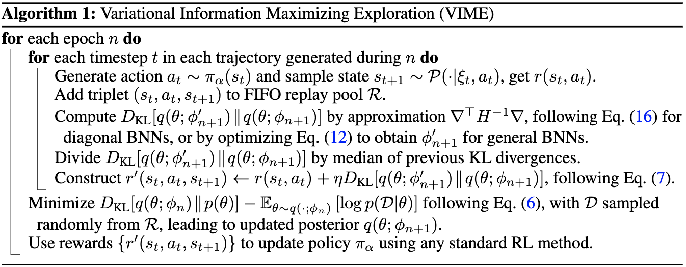
Algorithm
The overview of the algorithm is listed below (pasted from the original paper). In the implementation, where soft actor critic is used as baseline method, an agent is updated every step while the dynamics model posterior parameters $\phi$ is updated every episode.
References
[1] Houthooft R, Chen X, Duan Y, Schulman J, De Turck F, Abbeel P. Vime: Variational information maximizing exploration. InAdvances in Neural Information Processing Systems 2016 (pp. 1109-1117).
[2] Kingma DP, Salimans T, Welling M. Variational dropout and the local reparameterization trick. InAdvances in neural information processing systems 2015 (pp. 2575-2583).