2016年に作った資料を公開します。もう既にいろいろ古くなってる可能性が高いです。
参考資料
- Classifier comparison のサンプルプログラムを参考に。
- Scikit-learnのモデルをまとめてみた
-
k-近傍法
・ 決定木
・ランダムフォレスト
・AdaBoost
・ガウシアン・ナイーブ・ベイズ
・線形判別分析
・二次判別分析
より汎用的に使えるように改変してみました。
- タブ区切りのファイルを読み込み、PCAで次元圧縮し、様々な分類器で分類を行う流れを作ってみました。
def conduct_PCA(df):
    #import sklearn #機械学習のライブラリ
    from sklearn.decomposition import PCA #主成分分析器
    #主成分分析の実行
    pca = PCA()
    pca.fit(df.iloc[:, 1:5])
    # データを主成分空間に写像 = 次元圧縮
    feature = pca.transform(df.iloc[:, 1:5])
    # 既知ラベルの名前を、0, 1, 2 などの数字に置き換えます。
    target_names = []
    target = []
    for word in df[df.columns[5]]:
        if word not in target_names:
            target_names.append(word)
        target.append(target_names.index(word))
    return feature, target
def compare_classifiers(X, y):
    names = ["Nearest Neighbors", "Linear SVM", "RBF SVM", "Decision Tree",
             "Random Forest", "AdaBoost", "Naive Bayes", "Linear Discriminant Analysis",
             "Quadratic Discriminant Analysis"]

    classifiers = [
        KNeighborsClassifier(3),
        SVC(kernel="linear", C=0.025),
        SVC(gamma=2, C=1),
        DecisionTreeClassifier(max_depth=5),
        RandomForestClassifier(max_depth=5, n_estimators=10, max_features=1),
        AdaBoostClassifier(),
        GaussianNB(),
        LinearDiscriminantAnalysis(),
        QuadraticDiscriminantAnalysis()]

    figure = plt.figure(figsize=(12, 12))
    X = StandardScaler().fit_transform(X)
    X_train, X_test, y_train, y_test = train_test_split(X, y, test_size=.4)

    h = .02  # step size in the mesh
    x_min, x_max = X[:, 0].min() - .5, X[:, 0].max() + .5
    y_min, y_max = X[:, 1].min() - .5, X[:, 1].max() + .5
    xx, yy = np.meshgrid(np.arange(x_min, x_max, h),
                         np.arange(y_min, y_max, h))

    # just plot the dataset first
    cm = plt.cm.RdBu
    cm_bright = ListedColormap(['#FF0000', '#0000FF'])
    i = 1
    #ax = plt.subplot(3, len(classifiers) / 3, i)

    # iterate over classifiers
    for name, clf in zip(names, classifiers):
        #ax = plt.subplot(len(datasets), len(classifiers) + 1, i)
        ax = plt.subplot(3, len(classifiers) / 3, i)
        clf.fit(X_train, y_train)
        score = clf.score(X_test, y_test)

        # Plot the decision boundary. For that, we will assign a color to each
        # point in the mesh [x_min, m_max]x[y_min, y_max].
        if hasattr(clf, "decision_function"):
            Z = clf.decision_function(np.c_[xx.ravel(), yy.ravel()]) #[:, 1]
        else:
            Z = clf.predict_proba(np.c_[xx.ravel(), yy.ravel()])[:, 1]

        # Put the result into a color plot
        Z = Z.reshape(xx.shape)
        ax.contourf(xx, yy, Z, cmap=cm, alpha=.8)

        # Plot also the training points
        ax.scatter(X_train[:, 0], X_train[:, 1], c=y_train, cmap=cm_bright)
        # and testing points
        ax.scatter(X_test[:, 0], X_test[:, 1], c=y_test, cmap=cm_bright,
                   alpha=0.6)

        ax.set_xlim(xx.min(), xx.max())
        ax.set_ylim(yy.min(), yy.max())
        ax.set_xticks(())
        ax.set_yticks(())
        ax.set_title(name)
        ax.text(xx.max() - .3, yy.min() + .3, ('%.2f' % score).lstrip('0'),
                size=15, horizontalalignment='right')
        i += 1

figure.subplots_adjust(left=.02, right=.98)
plt.show()
# URL によるリソースへのアクセスを提供するライブラリをインポートする。
import urllib
# ウェブ上のリソースを指定する
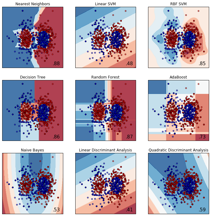
url = 'https://raw.githubusercontent.com/maskot1977/ipython_notebook/master/toydata/ToyData_linear.txt'
# 指定したURLからリソースをダウンロードし、名前をつける。
urllib.urlretrieve(url, 'ToyData_linear.txt')
import pandas as pd # データフレームワーク処理のライブラリをインポート
df = pd.read_csv("ToyData_linear.txt", sep='\t', na_values=".") # データの読み込み
feature, target = conduct_PCA(df)
X, y = feature[:, :2], target
compare_classifiers(X, y)
# URL によるリソースへのアクセスを提供するライブラリをインポートする。
import urllib
# ウェブ上のリソースを指定する
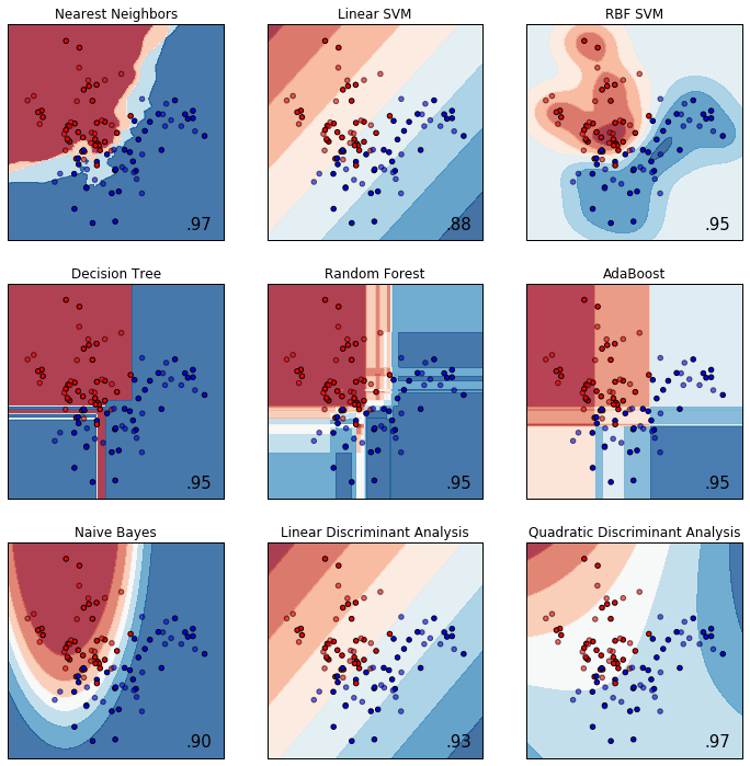
url = 'https://raw.githubusercontent.com/maskot1977/ipython_notebook/master/toydata/ToyData_moons.txt'
# 指定したURLからリソースをダウンロードし、名前をつける。
urllib.urlretrieve(url, 'ToyData_moons.txt')
import pandas as pd # データフレームワーク処理のライブラリをインポート
df = pd.read_csv("ToyData_moons.txt", sep='\t', na_values=".") # データの読み込み
feature, target = conduct_PCA(df)
X, y = feature[:, :2], target
compare_classifiers(X, y)
# URL によるリソースへのアクセスを提供するライブラリをインポートする。
import urllib
# ウェブ上のリソースを指定する
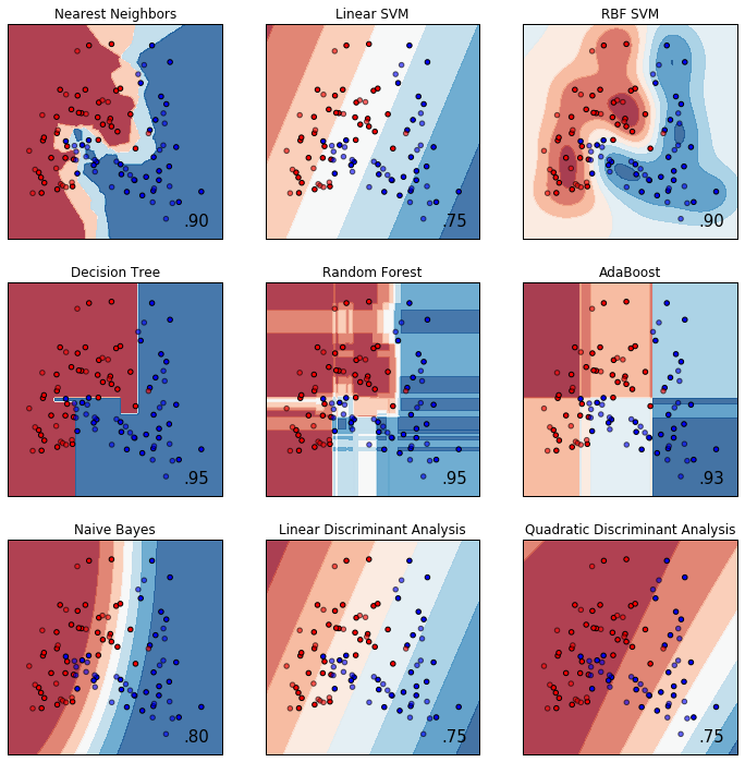
url = 'https://raw.githubusercontent.com/maskot1977/ipython_notebook/master/toydata/ToyData_circles.txt'
# 指定したURLからリソースをダウンロードし、名前をつける。
urllib.urlretrieve(url, 'ToyData_circles.txt')
import pandas as pd # データフレームワーク処理のライブラリをインポート
df = pd.read_csv("ToyData_circles.txt", sep='\t', na_values=".") # データの読み込み
feature, target = conduct_PCA(df)
X, y = feature[:, :2], target
compare_classifiers(X, y)
# URL によるリソースへのアクセスを提供するライブラリをインポートする。
import urllib
# ウェブ上のリソースを指定する
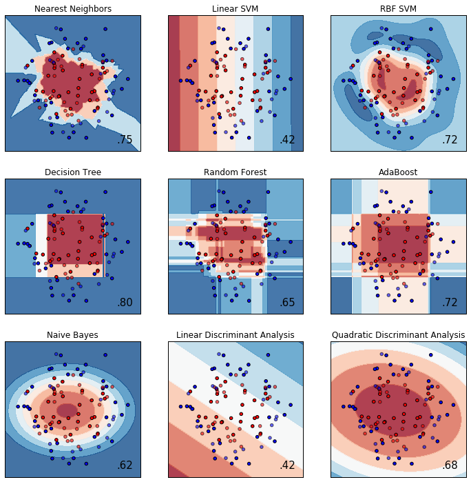
url = 'https://raw.githubusercontent.com/maskot1977/ipython_notebook/master/toydata/ToyData_gaussian_quantiles.txt'
# 指定したURLからリソースをダウンロードし、名前をつける。
urllib.urlretrieve(url, 'ToyData_gaussian_quantiles.txt')
import pandas as pd # データフレームワーク処理のライブラリをインポート
df = pd.read_csv("ToyData_gaussian_quantiles.txt", sep='\t', na_values=".") # データの読み込み
feature, target = conduct_PCA(df)
X, y = feature[:, :2], target
compare_classifiers(X, y)