Word2VecのCBOWをPyTorchで実装する

Word2Vecといっても、その実装には色んなバリエーションがあるそうですが、その中の CBOW (Continuous bag-of-words) ってのを PyTorch で実装してみました。あくまで勉強用であって、実用向きではありません。

学習済みモデルを Google Colaboratory に保存するための準備

次のようにして Google Colaboratory にマウントします。

from google.colab import drive
drive.mount('/content/drive')

Mounted at /content/drive

学習済みモデルを保存するためのディレクトリを指定します。なければ作ります。

import os

directory_path = './drive/MyDrive/word2vec3/'
if not os.path.exists(directory_path):
    os.makedirs(directory_path)

練習用データ

UCI の Machine-Learning Repository の SMS Spam Collection データセットを使います。与えられた文章から、それがスパムかどうかを判定する問題に用いますが、今回はスパムかどうかは判定せず、文章だけを使います。

import os
import requests
from zipfile import ZipFile
import io
import csv

save_file_name = os.path.join("temp", "temp_spam_data.csv")

# もしも元データがなければダウンロードする
if not os.path.exists("temp"):
    os.makedirs("temp")

if not os.path.isfile(save_file_name):
    zip_url = "http://archive.ics.uci.edu/ml/machine-learning-databases/00228/smsspamcollection.zip"
    r = requests.get(zip_url)
    z = ZipFile(io.BytesIO(r.content))
    file = z.read("SMSSpamCollection")

    text_data = file.decode()
    text_data = text_data.encode('ascii', errors='ignore')
    text_data = text_data.decode().split("\n")
    text_data = [x.split("\t") for x in text_data if len(x) > 1]

    with open(save_file_name, "w") as temp_output_file:
        writer = csv.writer(temp_output_file)
        writer.writerows(text_data)

# もし元データがあればそれを読み込む
else:
    text_data = []
    with open(save_file_name, "r") as temp_output_file:
        reader = csv.reader(temp_output_file)
        for row in reader:
            text_data.append(row)

texts = [x[1] for x in text_data]
target = [x[0] for x in text_data]

データの前処理

語彙の最終的なサイズを減らすために、テキストを正規化します。具体的には、テキストの大文字小文字の区別をなくしたり、数字を除いたり、余分なスペースを除いたり、句読点を除いたりします。

# 小文字に変換
texts = [x.lower() for x in texts]

# 数字を削除
texts = ["".join(c for c in x if c not in '0123456789') for x in texts]

# 余分なホワイトスペースを除去
texts = [" ".join(x.split()) for x in texts]

import string

# 句読点を削除
texts = ["".join(c for c in x if c not in string.punctuation) for x in texts]

ここでは、１つの文あたりの単語数を 25 とし、3 回以上出現しない単語も取り除きます。

class VocabularyProcessor:
    def __init__(self, sentence_size, min_frequency=3):
        self.sentence_size = sentence_size
        self.min_frequency = min_frequency
        self.freq = {}
        self.vocabulary_ = []
        self.vocab = {}
    
    def fit_transform(self, texts):
        freq = {}
        for sentence in texts:
            for word in sentence.split():
                if word not in freq.keys():
                    freq[word] = 0
                freq[word] += 1

        for k, v in freq.items():
            if v >= self.min_frequency:
                self.freq[k] = v

        self.vocabulary_ = self.freq.keys()

        transformed_texts = []
        for sentence in texts:
            transformed_sentence = []
            for word in sentence.split():
                if word in self.freq.keys():
                    if word not in self.vocab:
                        self.vocab[word] = len(self.vocab)

                    transformed_sentence.append(word)

                if len(transformed_sentence) >= self.sentence_size:
                    break

            transformed_sentence = " ".join(transformed_sentence)
            transformed_texts.append(transformed_sentence)
        return transformed_texts

sentence_size = 25
min_word_freq = 3

vocab_processor = VocabularyProcessor(sentence_size, min_frequency=min_word_freq)
texts = vocab_processor.fit_transform(texts)

N-gram の作成

文章中に隣接して現れる単語の列を作ります。ついでに vocab として、単語集を作ります。

n_grams = []
vocab = []
for text in texts:
    words = text.split()
    vocab += words
    n_grams += [([words[i], words[i+1], words[i+2], words[i+4], words[i+5], words[i+6]], words[i+3])
                for i in range(len(words) - 6)]

vocab = list(set(vocab))

vocab は保存しておいた方がいいですね。

import pickle

with open(directory_path + "vocab.pkl", 'wb') as f:
    pickle.dump(vocab, f)

CBOW (Continuous bag-of-words) モデル

次のように CBOW (Continuous bag-of-words) モデルを設計します。

import torch

class CBOW(torch.nn.Module):

    def __init__(self, vocab_size, embedding_dim, context_size):
        super(CBOW, self).__init__()
        self.embeddings = torch.nn.Embedding(vocab_size, embedding_dim)
        self.linear1 = torch.nn.Linear(context_size * embedding_dim, 128)
        self.linear2 = torch.nn.Linear(128, vocab_size)

    def forward(self, inputs):
        embeds = self.embeddings(inputs).view((1, -1))
        out = torch.nn.functional.relu(self.linear1(embeds))
        out = self.linear2(out)
        return out

学習

調整可能なパラメータとして、CONTEXT_SIZE を、文脈を考慮する前後の単語の合計数、EMBEDDING_DIM を、単語分散表現の次元数とします。

CONTEXT_SIZE = 6
EMBEDDING_DIM = 10

word_to_ix = {word: i for i, word in enumerate(vocab)}

losses = []
loss_function = torch.nn.CrossEntropyLoss()
model = CBOW(len(vocab), EMBEDDING_DIM, CONTEXT_SIZE)
optimizer = torch.optim.SGD(model.parameters(), lr=0.001)

学習開始。学習途中のモデルも保存するようにしています。

for epoch in range(400):
    !date
    total_loss = torch.Tensor([0])
    for context, target in n_grams:
        context_idxs = [word_to_ix[w] for w in context]
        context_var = torch.autograd.Variable(torch.LongTensor(context_idxs))
        model.zero_grad()
        output = model(context_var)
        loss = loss_function(output, torch.autograd.Variable(torch.LongTensor([word_to_ix[target]])))
        loss.backward()
        optimizer.step()
        total_loss += loss.data
    losses.append(total_loss.detach().numpy()[0])
    print(epoch, total_loss)

    PATH = directory_path + "model_{}.pth".format(epoch)
    torch.save(model.state_dict(), PATH)

学習曲線は次のようになりました。

import matplotlib.pyplot as plt

plt.plot(losses)
plt.xlabel("epoch")
plt.ylabel("loss")
plt.show()

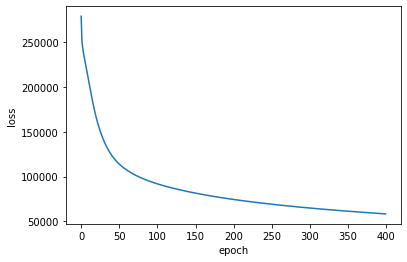
まだ学習し足りない気がしますが、このへんで終わりとします。いちおうロスの履歴も保存しときます。

import pickle

with open(directory_path + "losses.pkl", 'wb') as f:
    pickle.dump(losses, f)

CBOWモデルの構成

今回使ったCBOWモデルは次のような構成でした。

model

CBOW(
  (embeddings): Embedding(2694, 10)
  (linear1): Linear(in_features=60, out_features=128, bias=True)
  (linear2): Linear(in_features=128, out_features=2694, bias=True)
)

その中の embeddings が、単語数 x 埋め込み次元数 の形の行列、つまり単語分散表現。

model.embeddings.weight

Parameter containing:
tensor([[ 0.1757,  2.1936,  1.1479,  ..., -0.4144, -0.7548,  0.3695],
        [ 0.1962,  0.0238,  1.1729,  ..., -2.3863,  0.4950, -0.1202],
        [ 0.9316,  0.7451,  0.5241,  ...,  0.0532,  0.1612, -0.2888],
        ...,
        [-0.6087,  1.9787,  0.4039,  ...,  0.3821,  0.6576,  1.8304],
        [-1.2499, -0.4358, -1.4592,  ...,  0.6641, -0.8658, -1.0650],
        [ 0.4118, -0.2603, -1.9144,  ..., -1.2599,  0.1849,  0.6056]],
       requires_grad=True)

word2vec というと普通は機械学習モデルを指すと思いますが、ここでは word2vec ＝「単語をベクトルに変換するもの」＝「単語分散表現の行列」という変数名にしました（乱暴）

word2vec = model.embeddings.weight.detach().numpy()
word2vec

array([[ 0.17574234,  2.193559  ,  1.1479073 , ..., -0.41436067,
        -0.7548341 ,  0.36947948],
       [ 0.19621728,  0.02384255,  1.1728823 , ..., -2.38634   ,
         0.49504647, -0.12015778],
       [ 0.9316455 ,  0.74507606,  0.5240704 , ...,  0.05318468,
         0.16119353, -0.2887744 ],
       ...,
       [-0.60866654,  1.9787219 ,  0.4038656 , ...,  0.38205254,
         0.65760624,  1.8303967 ],
       [-1.249858  , -0.4358453 , -1.4592329 , ...,  0.6640799 ,
        -0.8657619 , -1.0649782 ],
       [ 0.41184828, -0.26025063, -1.914422  , ..., -1.259887  ,
         0.18489367,  0.60559577]], dtype=float32)

単語分散表現を Isomap で可視化

word2vec を自作してみました系の記事ではよく、ある単語とよく似ている単語を取り出してます。ですがそれを１つ２つ例示しただけではピンと来ないなと思ったので、 Isomap を使って可視化してみたいと思います。下の図では、各単語が丸で表現されています。

from sklearn.manifold import Isomap
import matplotlib.pyplot as plt

mapper = Isomap()
embedding = mapper.fit_transform(word2vec)
plt.scatter(embedding[:, 0], embedding[:, 1], alpha=0.5)
plt.colorbar()
plt.show()

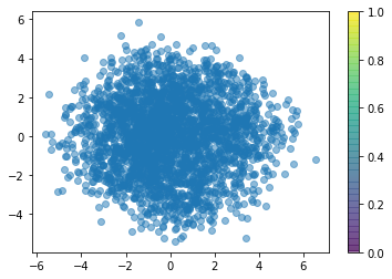
はい、もっとピンと来ませんね。

距離が近い（＝似ている）単語だけをいくつか抜き出して図示するようにしましょう。

import numpy as np

word_pair = []
for i1 in range(len(word2vec)):
    A = word2vec[i1]
    for i2 in range(len(word2vec)):
        if i1 >= i2: continue
        B = word2vec[i2]
        dist = np.sum((A - B)**2)
        word_pair.append([vocab[i1], vocab[i2], dist])

word_pair.sort(key=lambda x:x[2])

selected_words = []
for pair in word_pair[:100]:
    selected_words.append(word_to_ix[pair[0]])
    selected_words.append(word_to_ix[pair[1]])

selected_words = list(set(selected_words))
selected_words.sort()

次のようになりました。

from sklearn.manifold import Isomap
import matplotlib.pyplot as plt

mapper = Isomap()
embedding = mapper.fit_transform(word2vec[selected_words, :])
fig, axes = plt.subplots(nrows=1, ncols=1, figsize=(8, 8))
for i in range(len(embedding)):
    axes.text(embedding[i, 0], embedding[i, 1], vocab[selected_words[i]], size=50, alpha=0.5)
axes.axis("off")
plt.show()

beautiful と dirty が近くに来てるのは、なんか良い感じかもしれない。あとは sunday と tomorrow とか。ん？ pizza と cream が近くにあるぞ？

A - B = C - D

word2vec の醍醐味といえば、単語間で A - B = C - D のような演算ができることじゃないですか。やってみましたよ。

word_A = "drink"
word_B = "drunk"
query_vec = word2vec[word_to_ix[word_A]] - word2vec[word_to_ix[word_B]] 

search_results = []
for i3 in range(len(word2vec)):
    C = word2vec[i3]
    for i4 in range(len(word2vec)):
        D = word2vec[i4]
        target_vec = C - D
        dist = np.sum((query_vec - target_vec)**2)
        search_results.append([vocab[i3], vocab[i4], dist])

search_results.sort(key=lambda x:x[2])
search_results[:10]

[['drink', 'drunk', 0.0],
 ['drink', 'ym', 1.2704575],
 ['minute', 'ho', 1.5435413],
 ['ron', 'footprints', 1.8065212],
 ['picked', 'ho', 1.8251992],
 ['dirty', 'drunk', 1.8444525],
 ['house', 'gotta', 1.8611782],
 ['hotel', 'terms', 1.8623177],
 ['pound', 'bad', 1.914198],
 ['series', 'parents', 1.9171268]]

学習データも小さいし、学習も雑だし、埋め込み次元数も小さいし、無理っすね...