PuLPで解く最適割当問題と最適輸送問題

「PuLPで解く線形計画法と連立方程式とナップサック問題」の続編です。今度は最適割当問題と最適輸送問題を取り扱います。

インストール

!pip install pulp

Collecting pulp
[?25l  Downloading https://files.pythonhosted.org/packages/14/c4/0eec14a0123209c261de6ff154ef3be5cad3fd557c084f468356662e0585/PuLP-2.4-py3-none-any.whl (40.6MB)
[K     |████████████████████████████████| 40.6MB 75kB/s 
[?25hCollecting amply>=0.1.2
  Downloading https://files.pythonhosted.org/packages/f3/c5/dfa09dd2595a2ab2ab4e6fa7bebef9565812722e1980d04b0edce5032066/amply-0.1.4-py3-none-any.whl
Requirement already satisfied: docutils>=0.3 in /usr/local/lib/python3.7/dist-packages (from amply>=0.1.2->pulp) (0.17.1)
Requirement already satisfied: pyparsing in /usr/local/lib/python3.7/dist-packages (from amply>=0.1.2->pulp) (2.4.7)
Installing collected packages: amply, pulp
Successfully installed amply-0.1.4 pulp-2.4

必要なライブラリのインポート

import pulp
import numpy as np
import matplotlib.pyplot as plt

最適割当問題

一対一の最適割当問題

「工場」と「店舗」が同じ数だけ存在するものとします。工場と店舗の契約は一対一しか認めないものとします。

次のようにして、工場の所在地の X 座標と Y 座標を決めます。

n_factory = 10
factories = np.random.rand(n_factory, 2)
factories

array([[0.66483621, 0.03770088],
       [0.3882542 , 0.64300815],
       [0.28063954, 0.18537062],
       [0.7573773 , 0.45668832],
       [0.22048815, 0.07562346],
       [0.77617785, 0.22661663],
       [0.06343604, 0.10612717],
       [0.48937361, 0.45101889],
       [0.32021719, 0.53954648],
       [0.62202243, 0.45476437]])

同様にして、店舗の所在地の X 座標と Y 座標を決めます。

n_shop = 10
shops = np.random.rand(n_shop, 2) 
shops

array([[9.94721474e-01, 4.82056184e-01],
       [1.06774138e-01, 1.85362411e-01],
       [2.03526252e-01, 2.53051660e-01],
       [6.35310607e-01, 8.15960070e-01],
       [5.68434066e-01, 1.18073980e-01],
       [6.54962725e-01, 4.53184395e-01],
       [3.94012302e-01, 9.15773476e-01],
       [3.99162185e-01, 3.72698106e-01],
       [5.93860619e-01, 9.09725408e-01],
       [4.70633167e-04, 3.99793227e-01]])

工場と店舗の位置関係を図示すると次のようになります。

plt.figure(figsize=(8, 8))

plt.scatter(
    factories[:, 0], factories[:, 1], marker="s", s=100, alpha=0.8, label="factories"
)
for i, (x, y) in enumerate(factories):
    plt.text(x, y, i)

plt.scatter(shops[:, 0], shops[:, 1], marker="^", s=100, alpha=0.8, label="shops")
for i, (x, y) in enumerate(shops):
    plt.text(x, y, i)

plt.legend()
plt.show()

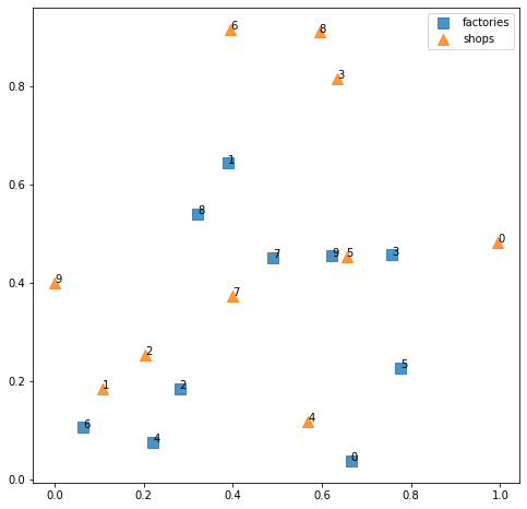
契約のコストは、工場から店舗までのユークリッド距離の２乗に比例するものとします。

cost = np.empty((len(factories), len(shops)))
for i in range(len(factories)):
    for j in range(len(shops)):
        distance = (factories[i][0] - shops[j][0]) **2 + (factories[i][1] - shops[j][1]) **2
        cost[i, j] = distance

コストは次のような２次元配列として表現されます。

cost

array([[0.30627593, 0.3332372 , 0.25918283, 0.60655913, 0.01575321,
        0.17272404, 0.84435707, 0.18280583, 0.76546431, 0.57249248],
       [0.3937081 , 0.28867065, 0.18619048, 0.09094924, 0.30802067,
        0.1071665 , 0.07443408, 0.07318651, 0.11341209, 0.20952959],
       [0.59793533, 0.03022918, 0.01052718, 0.52343462, 0.08735453,
        0.21184206, 0.54634171, 0.0491392 , 0.6227973 , 0.12447167],
       [0.05697578, 0.49690223, 0.34821888, 0.14397647, 0.15035922,
        0.01050102, 0.3427933 , 0.13537243, 0.23198031, 0.57614476],
       [0.76462479, 0.02497351, 0.03176847, 0.72017596, 0.12286841,
        0.33132041, 0.73596267, 0.12017775, 0.83513305, 0.15349374],
       [0.11301068, 0.44980324, 0.32862866, 0.36716927, 0.05493898,
        0.06602606, 0.62098766, 0.16348061, 0.49987717, 0.63171181],
       [1.00861518, 0.00815641, 0.04121207, 0.83090327, 0.25516573,
        0.47035254, 0.76480781, 0.18377211, 0.92712036, 0.0902044 ],
       [0.25633977, 0.21695572, 0.12089974, 0.15447967, 0.11710287,
        0.02742444, 0.2250906 , 0.01427225, 0.2213292 , 0.24165019],
       [0.45826116, 0.1710043 , 0.09569606, 0.17568833, 0.23925069,
        0.11951298, 0.14699247, 0.03407069, 0.21191316, 0.12176884],
       [0.13964942, 0.33805822, 0.21582707, 0.13063891, 0.11623213,
        0.00108756, 0.26451802, 0.05640156, 0.20778264, 0.38934847]])

工場から店舗を結ぶ「辺」 (edge) を契約関係とみなし、工場と店舗の全組み合わせについて作成します。この辺は 0 か 1 かの binary matrix として定義します。

edges = np.array(pulp.LpVariable.matrix('edge', (range(len(factories)), range(len(shops))), cat='Binary'))

今回の最適割当問題は、契約によって生じるコストの最小化を目指すものとします。

prob = pulp.LpProblem('optimal_assignment_problem', sense=pulp.LpMinimize)

最小化したい関数は、コストと辺の積和として表現できます。

prob += pulp.lpDot(cost.flatten(), edges.flatten())

制約条件は、１つの工場が契約している店舗は１つだけ、１つの店舗が契約している工場は１つだけ、ということになります。

for i in range(len(shops)):
    prob += pulp.lpSum(edges[i]) == 1
    prob += pulp.lpSum(edges[:, i]) == 1

ソルバー実行。

result = prob.solve()

最適解が求まったかどうか。

pulp.LpStatus[result]

'Optimal'

求まった最適解を図示すると次のようになります。

plt.figure(figsize=(8, 8))

plt.title("Optimal Value = {}".format(pulp.value(prob.objective)))
plt.scatter(factories[:, 0], factories[:, 1], 
            marker='s', s=100, alpha=0.8, label="factories")
for i, (x, y) in enumerate(factories):
    plt.text(x, y, i)

plt.scatter(shops[:, 0], shops[:, 1], 
            marker='^', s=100, alpha=0.8, label="shops")
for i, (x, y) in enumerate(shops):
    plt.text(x, y, i)

for i in range(len(shops)):
    for j in range(len(shops)):
        if edges[i, j].varValue == 1:
            x1, y1 = factories[i]
            x2, y2 = shops[j]
            plt.plot([x1, x2], [y1, y2], c="lightblue")

plt.legend()
plt.show()

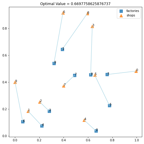
全体としての最適化を目指したため、必ずしも最短距離の工場・店舗が結ばれたわけではないことが分かります。

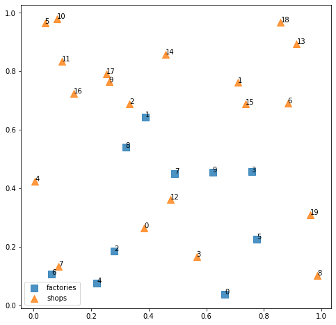
一対二の最適割当問題

今度は、工場と店舗が１：２であるとして、１つの工場は必ず２つの店舗と契約するという条件で、コスト最小化を目指しましょう。

店舗のデータを更新します。

n_shop = 20
shops = np.random.rand(n_shop, 2) 
shops

array([[0.38487129, 0.26475778],
       [0.70912289, 0.76126158],
       [0.33270909, 0.68937289],
       [0.56633054, 0.16716666],
       [0.00529438, 0.4245301 ],
       [0.03945408, 0.96407753],
       [0.88265877, 0.6904835 ],
       [0.08655507, 0.13338917],
       [0.98578141, 0.10256008],
       [0.26187659, 0.76359637],
       [0.08068534, 0.98000186],
       [0.09791736, 0.83433169],
       [0.47502831, 0.36237432],
       [0.91395895, 0.89364293],
       [0.45866741, 0.85816628],
       [0.73534453, 0.68746109],
       [0.13942188, 0.72401213],
       [0.25260789, 0.79108937],
       [0.85839067, 0.96682538],
       [0.96130838, 0.30919617]])

工場と店舗の位置関係です。

plt.figure(figsize=(8, 8))

plt.scatter(factories[:, 0], factories[:, 1], 
            marker='s', s=100, alpha=0.8, label="factories")
for i, (x, y) in enumerate(factories):
    plt.text(x, y, i)

plt.scatter(shops[:, 0], shops[:, 1], 
            marker='^', s=100, alpha=0.8, label="shops")
for i, (x, y) in enumerate(shops):
    plt.text(x, y, i)

plt.legend()
plt.show()

基本的には、一対一の場合と同じように書けます。

cost = np.empty((len(factories), len(shops)))
for i in range(len(factories)):
    for j in range(len(shops)):
        distance = (factories[i][0] - shops[j][0]) **2 + (factories[i][1] - shops[j][1]) **2
        cost[i, j] = distance

edges = np.array(pulp.LpVariable.matrix('edge', (range(len(factories)), range(len(shops))), cat='Binary'))

prob = pulp.LpProblem('割り当て問題', sense=pulp.LpMinimize)
prob += pulp.lpDot(cost.flatten(), edges.flatten())

変更すべき部分はこちらになります。

for i in range(len(factories)):
    prob += pulp.lpSum(edges[i]) == 2

for i in range(len(shops)):
    prob += pulp.lpSum(edges[:, i]) == 1

ソルバー実行。

result = prob.solve()
pulp.LpStatus[result]

'Optimal'

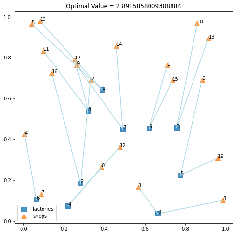
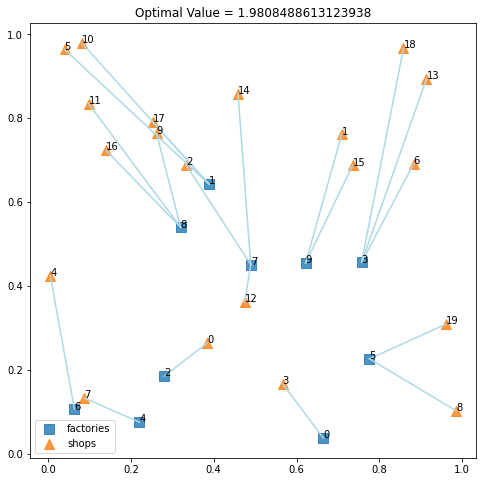
求まった最適解を図示すると次のようになります。

plt.figure(figsize=(8, 8))

plt.title("Optimal Value = {}".format(pulp.value(prob.objective)))
plt.scatter(factories[:, 0], factories[:, 1], 
            marker='s', s=100, alpha=0.8, label="factories")
for i, (x, y) in enumerate(factories):
    plt.text(x, y, i)

plt.scatter(shops[:, 0], shops[:, 1], 
            marker='^', s=100, alpha=0.8, label="shops")
for i, (x, y) in enumerate(shops):
    plt.text(x, y, i)

for i in range(len(factories)):
    for j in range(len(shops)):
        if edges[i, j].varValue == 1:
            x1, y1 = factories[i]
            x2, y2 = shops[j]
            plt.plot([x1, x2], [y1, y2], c="lightblue")

plt.legend()
plt.show()

一対多の最適割当問題

と、いうことで、少し変更するだけで一対多や多対多の最適割当問題に拡張できます。次は、１つの工場は１〜３の店舗と契約することとし、１つの店舗は１つの工場としか契約できないものとした場合です。

prob = pulp.LpProblem('optimum_assignment_problem', sense=pulp.LpMinimize)
prob += pulp.lpDot(cost.flatten(), edges.flatten())

for i in range(len(factories)):
    prob += pulp.lpSum(edges[i]) <= 3
    prob += pulp.lpSum(edges[i]) >= 1

for i in range(len(shops)):
    prob += pulp.lpSum(edges[:, i]) == 1

result = prob.solve()
pulp.LpStatus[result]

'Optimal'

plt.figure(figsize=(8, 8))

plt.title("Optimal Value = {}".format(pulp.value(prob.objective)))
plt.scatter(factories[:, 0], factories[:, 1], 
            marker='s', s=100, alpha=0.8, label="factories")
for i, (x, y) in enumerate(factories):
    plt.text(x, y, i)

plt.scatter(shops[:, 0], shops[:, 1], 
            marker='^', s=100, alpha=0.8, label="shops")
for i, (x, y) in enumerate(shops):
    plt.text(x, y, i)

for i in range(len(factories)):
    for j in range(len(shops)):
        if edges[i, j].varValue == 1:
            x1, y1 = factories[i]
            x2, y2 = shops[j]
            plt.plot([x1, x2], [y1, y2], c="lightblue")

plt.legend()
plt.show()

最適輸送問題

最適輸送問題は、最適割当問題と何となく似てますがもっと複雑な問題設定になります。

図がごちゃごちゃすると見にくいので、工場の数を減らしましょう。

n_factory = 4
factories = np.random.rand(n_factory, 2)
factories

array([[0.76522304, 0.17828041],
       [0.96573477, 0.60239741],
       [0.36347754, 0.09666514],
       [0.31981222, 0.83556475]])

店舗の数も減らしておきます。

n_shop = 10
shops = np.random.rand(n_shop, 2) 
shops

array([[0.58184441, 0.60161301],
       [0.12017488, 0.19453957],
       [0.8832619 , 0.39381807],
       [0.13381321, 0.94035459],
       [0.85377643, 0.45427797],
       [0.23022818, 0.0089919 ],
       [0.88793818, 0.81329285],
       [0.83551052, 0.00194519],
       [0.89053601, 0.19966076],
       [0.91336169, 0.26206935]])

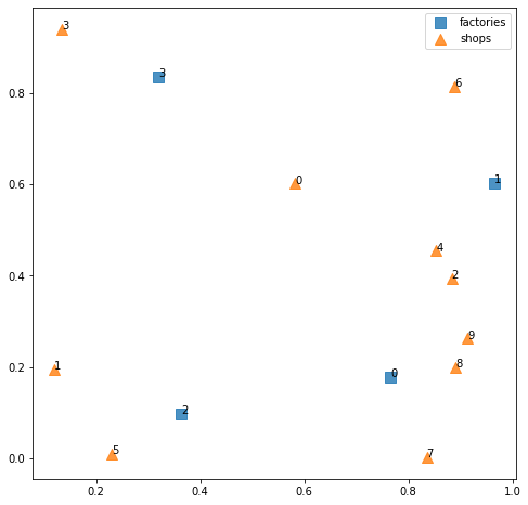
工場と店舗の位置関係は次のようになります。

plt.figure(figsize=(8, 8))

plt.scatter(factories[:, 0], factories[:, 1], 
            marker='s', s=100, alpha=0.8, label="factories")
for i, (x, y) in enumerate(factories):
    plt.text(x, y, i)

plt.scatter(shops[:, 0], shops[:, 1], 
            marker='^', s=100, alpha=0.8, label="shops")
for i, (x, y) in enumerate(shops):
    plt.text(x, y, i)

plt.legend()
plt.show()

最適輸送問題で新たに加わった設定は、工場の「供給量」と店舗の「需要量」です。

supply = np.random.rand(n_factory)
supply = supply / supply.sum()
supply

array([0.33092066, 0.08212874, 0.27954164, 0.30740897])

demand = np.random.rand(n_shop)
demand = demand / demand.sum()
demand

array([0.10084757, 0.1143852 , 0.05213198, 0.1259985 , 0.09829416,
       0.05231464, 0.14107469, 0.11664057, 0.12381253, 0.07450014])

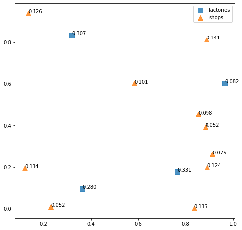
工場の「供給量」の総和と、店舗の「需要量」の総和は同じになるようにしています。

では、今まで工場と店舗の ID を図示していましたが、次からは工場の「供給量」と店舗の「需要量」を図示することにしましょう。

plt.figure(figsize=(8, 8))

plt.scatter(factories[:, 0], factories[:, 1], 
            marker='s', s=100, alpha=0.8, label="factories")
for (x, y), z in zip(factories, supply):
    plt.text(x, y, "{:.3f}".format(z))

plt.scatter(shops[:, 0], shops[:, 1], 
            marker='^', s=100, alpha=0.8, label="shops")
for (x, y), z in zip(shops, demand):
    plt.text(x, y, "{:.3f}".format(z))

plt.legend()
plt.show()

この需要と供給をマッチングさせるように契約します。コストは、「工場と店舗の距離の２乗」と「輸送量」の積和とします。このコストが最小となるような輸送の割り当てを決定するわけです。

これを計算するためにコストのデータを用意しますが、今回は次のようなデータ構造にした方が便利なのでそうしましょう。

cost = {}
for i in range(len(supply)):
    for j in range(len(demand)):
        distance = (factories[i][0] - shops[j][0]) **2 + (factories[i][1] - shops[j][1]) **2
        cost[(i, j)] = distance

cost

{(0, 0): 0.21283821653690962,
 (0, 1): 0.4163514917992923,
 (0, 2): 0.06038965701867623,
 (0, 3): 0.9794354278613777,
 (0, 4): 0.08401635732508601,
 (0, 5): 0.31487809660360483,
 (0, 6): 0.41829980652299564,
 (0, 7): 0.03603443837319058,
 (0, 8): 0.016160460359886435,
 (0, 9): 0.028965648368420322,
 (1, 0): 0.14737242116569105,
 (1, 1): 0.8813195594267481,
 (1, 2): 0.05030711714920501,
 (1, 3): 0.8063085360692637,
 (1, 4): 0.034474040522258595,
 (1, 5): 0.8931000459221654,
 (1, 6): 0.0505291936967214,
 (1, 7): 0.3775012296001897,
 (1, 8): 0.1678516619580682,
 (1, 9): 0.1185661306516755,
 (2, 0): 0.30265644843971146,
 (2, 1): 0.06877558846435997,
 (2, 2): 0.3584756439215455,
 (2, 3): 0.7645575847472579,
 (2, 4): 0.3682799372477021,
 (2, 5): 0.025441987916108882,
 (2, 6): 0.7886142361657633,
 (2, 7): 0.23178700305957142,
 (2, 8): 0.28839873094305424,
 (2, 9): 0.32973113817323735,
 (3, 0): 0.12339428619393354,
 (3, 1): 0.45076835761577666,
 (3, 2): 0.5126156666248091,
 (3, 3): 0.04557654172450732,
 (3, 4): 0.430497385891638,
 (3, 5): 0.6912479730796491,
 (3, 6): 0.32326314293055464,
 (3, 7): 0.9608663079602262,
 (3, 8): 0.730099522992236,
 (3, 9): 0.6811979546467961}

では最適化計算を実行します。厳密にやると解が見つからない場合があるので不等号を入れたりしてます。

edges = {(i,j): pulp.LpVariable("edge({},{})".format(i,j), lowBound=0, upBound=demand[j]) for i,j in cost}

prob = pulp.LpProblem(name='optimal_transportation_problem', sense=pulp.LpMinimize)

prob += pulp.lpSum([edges[i,j] * cost[i,j] for i,j in cost])

for i, si in enumerate(supply):
    prob += pulp.lpSum([edges[i,j] for j in range(len(demand))]) <= si

for j, dj in enumerate(demand):
    prob += pulp.lpSum([edges[i,j] for i in range(len(supply))]) == dj

result = prob.solve()
pulp.LpStatus[result]

'Optimal'

次のように結果が得られました。青い文字は工場から店舗までの輸送量になります。輸送量がある程度より小さい場合は輸送量ゼロとみなしています。

plt.figure(figsize=(8, 8))

plt.title("Optimal Value = {}".format(pulp.value(prob.objective)))

plt.scatter(factories[:, 0], factories[:, 1], 
            marker='s', s=100, alpha=0.8, label="factories")
for (x, y), z in zip(factories, supply):
    plt.text(x, y, "{:.3f}".format(z))

plt.scatter(shops[:, 0], shops[:, 1], 
            marker='^', s=100, alpha=0.8, label="shops")
for (x, y), z in zip(shops, demand):
    plt.text(x, y, "{:.3f}".format(z))

plt.legend()
for k, v in edges.items():
    x1, y1 = factories[k[0]]
    x2, y2 = shops[k[1]]
    if v.varValue > 1e-4:
        plt.plot([x1, x2], [y1, y2], c="lightblue")
        plt.text((x1 + x2) / 2, (y1 + y2) / 2, "{:.3f}".format(v.varValue), c="blue")

plt.show()

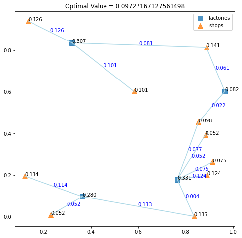
制約条件の式を PuLP の作法に合うように書いたり、厳密な最適解が見つからない場合に条件を微妙に緩めたりするのにちょっとしたコツが必要ですね。