準備

必要なライブラリのインポート

# 数値計算やデータフレーム操作に関するライブラリをインポートする
import numpy as np
import pandas as pd

# URL によるリソースへのアクセスを提供するライブラリをインポートする。
import urllib.request

# 図やグラフを図示するためのライブラリをインポートする。
import matplotlib.pyplot as plt
%matplotlib inline

# 線形回帰を行なうライブラリ
from sklearn import linear_model

データのダウンロードと整形

赤ワインのデータ

データは UC Irvine Machine Learning Repository から取得したものを少し改変しました。

赤ワイン https://raw.githubusercontent.com/chemo-wakate/tutorial-6th/master/beginner/data/winequality-red.txt

白ワイン https://raw.githubusercontent.com/chemo-wakate/tutorial-6th/master/beginner/data/winequality-white.txt

fixed acidity : 不揮発酸濃度（ほぼ酒石酸濃度）
volatile acidity : 揮発酸濃度（ほぼ酢酸濃度）
citric acid : クエン酸濃度
residual sugar : 残存糖濃度
chlorides : 塩化物濃度
free sulfur dioxide : 遊離亜硫酸濃度
total sulfur dioxide : 亜硫酸濃度
density : 密度
pH : pH
sulphates : 硫酸塩濃度
alcohol : アルコール度数
quality (score between 0 and 10) : 0-10 の値で示される品質のスコア

# ウェブ上のリソースを指定する
url = 'https://raw.githubusercontent.com/chemo-wakate/tutorial-6th/master/beginner/data/winequality-red.txt'
# 指定したURLからリソースをダウンロードし、名前をつける。
urllib.request.urlretrieve(url, 'winequality-red.txt')

('winequality-red.txt', <http.client.HTTPMessage at 0x11de96198>)

# データの読み込み
df = pd.read_csv('winequality-red.txt', sep='\t', index_col=0)

df.head()

	fixed acidity	volatile acidity	citric acid	residual sugar	chlorides	free sulfur dioxide	total sulfur dioxide	density	pH	sulphates	alcohol	quality
0	7.4	0.70	0.00	1.9	0.076	11.0	34.0	0.9978	3.51	0.56	9.4	5
1	7.8	0.88	0.00	2.6	0.098	25.0	67.0	0.9968	3.20	0.68	9.8	5
2	7.8	0.76	0.04	2.3	0.092	15.0	54.0	0.9970	3.26	0.65	9.8	5
3	11.2	0.28	0.56	1.9	0.075	17.0	60.0	0.9980	3.16	0.58	9.8	6
4	7.4	0.70	0.00	1.9	0.076	11.0	34.0	0.9978	3.51	0.56	9.4	5

品質の良いワインだけ考える

# 品質の良いワインだけ選択し df1 に入れる
df1 = df[df['quality'] > 6]

df1.head()

	fixed acidity	volatile acidity	citric acid	residual sugar	chlorides	free sulfur dioxide	total sulfur dioxide	density	pH	sulphates	alcohol	quality
7	7.3	0.65	0.00	1.2	0.065	15.0	21.0	0.9946	3.39	0.47	10.0	7
8	7.8	0.58	0.02	2.0	0.073	9.0	18.0	0.9968	3.36	0.57	9.5	7
16	8.5	0.28	0.56	1.8	0.092	35.0	103.0	0.9969	3.30	0.75	10.5	7
37	8.1	0.38	0.28	2.1	0.066	13.0	30.0	0.9968	3.23	0.73	9.7	7
62	7.5	0.52	0.16	1.9	0.085	12.0	35.0	0.9968	3.38	0.62	9.5	7

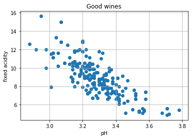
pH と不揮発酸濃度との関係を考える

X = df1['pH'].values
Y = df1['fixed acidity'].values

plt.title('Good wines')
plt.scatter(X, Y)
plt.xlabel('pH')
plt.ylabel('fixed acidity')
plt.grid()
plt.show()

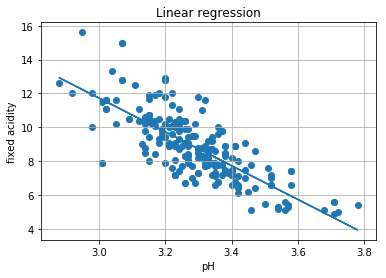
scikit-learn を用いた線形単回帰分析

from sklearn import linear_model
clf = linear_model.LinearRegression()
X2 = [[x] for x in X]
clf.fit(X2, Y) # 予測モデルを作成

# 散布図
plt.scatter(X2, Y)

# 回帰直線
plt.title('Linear regression')
plt.plot(X2, clf.predict(X2))
plt.xlabel('pH')
plt.ylabel('fixed acidity')
plt.grid()
plt.show()

print("回帰係数= ", clf.coef_)
print("切片= ", clf.intercept_)
print("決定係数= ", clf.score(X2, Y))

回帰係数=  [-9.985041]
切片=  41.685825856217654
決定係数=  0.5948141769596296

演習：上の結果を scikit-learn を使わず再現しよう

平均値

# 平均値を求める関数を作ろう
def average(list):

print(average(X))
print(average(Y))

3.2888018433179704
8.84700460829493

分散

# 分散を求める関数を作ろう
def variance(list):

print(variance(X))
print(variance(Y))

0.023753403130242778
3.9814772027437417

標準偏差

# 標準偏差を求める関数を作ろう
import math
def standard_deviation(list):

print(standard_deviation(X))
print(standard_deviation(Y))

0.1541213908912153
1.9953639273936326

共分散

# 共分散 = 偏差積の平均 （偏差値、ではありません。偏差積、です）を作ろう
def covariance(list1, list2):

print(covariance(X, Y))

-0.23717870415596012

相関係数

# 相関係数 = 共分散を list1, list2 の標準偏差で割ったものを作ろう
def correlation(list1, list2):

print(correlation(X, Y))

-0.7712419704344603

回帰直線

# 回帰直線の傾き＝相関係数＊（（yの標準偏差）／（xの標準偏差））を求める関数を作ろう
def a_fit(xlist, ylist):

print(a_fit(X, Y))

-9.985041000461308

# y切片＝yの平均－（傾き＊xの平均）を求める関数を作ろう
def b_fit(xlist, ylist):

print(b_fit(X, Y))

41.68582585621759

# 回帰直線の式
print("y = ax + b; (a, b) = ({}, {})".format(a_fit(X, Y), b_fit(X, Y)))

y = ax + b; (a, b) = (-9.985041000461308, 41.68582585621759)

# 回帰式を作ろう
def f(x):

f(3.5)

6.738182354603012

決定係数

# 決定係数を求める関数を作ろう
def r2(X, Y):

r2(X,Y)

0.5948141769596293

# 散布図と回帰直線を描いてみよう

回帰係数=  -9.985041000461308
切片=  41.68582585621759
決定係数=  0.5948141769596293

補足：計算速度の改善の話

講義中に「回帰式を作ろう」の部分で

def f(x):
    return a_fit(X, Y) * x + b_fit(X, Y)

と書いてしまいましたが、それは良くなかったですね。回帰係数と切片は定数なので、本来は一度だけ計算すれば済むものなのですが、これだと、f(x) を呼び出すたびに回帰係数と切片を再計算しなければならなくなるため、決定係数の計算が大変遅くなります。試しに品質の良い赤ワインのデータで時間を計測してみると

%timeit r2(X,Y)

328 ms ± 9.09 ms per loop (mean ± std. dev. of 7 runs, 1 loop each)

もかかってしまいました。そこで、回帰係数と切片を再計算しなくて済むように改良すると

afit = a_fit(X, Y)
bfit = b_fit(X, Y)
def f(x):
    return afit * x + bfit

%timeit r2(X,Y)

6.68 ms ± 297 µs per loop (mean ± std. dev. of 7 runs, 100 loops each)

だいぶ改善されました。

課題

以下の例について、scikit-learnを使わずに線形単回帰を行ない、散布図と回帰直線を描画し、回帰係数・切片・決定係数を表示してください。また、scikit-learnを使った結果と比較することにより検算してください。

品質の良い赤ワインの密度(density)から不揮発酸濃度(fixed acidity)を予測
品質の良くない赤ワインのpHから不揮発酸濃度(fixed acidity)を予測
品質の良くない赤ワインの密度 (density) から不揮発酸濃度 (fixed acidity) を予測
品質の良い白ワインのpHから不揮発酸濃度(fixed acidity)を予測
品質の良い白ワインの密度(density)から不揮発酸濃度(fixed acidity)を予測
品質の良くない白ワインのpHから不揮発酸濃度(fixed acidity)を予測
品質の良くない白ワインの密度(density)から不揮発酸濃度(fixed acidity)を予測

ただし、「品質が良くない」 = 「quality が 5 未満」とします。

以上の解析から、赤ワイン・白ワインの品質と、pH、密度、不揮発酸濃度の関係について考察してください。

線形単回帰を Python で理解する

準備