CNNで画像分類をやってみました

AIってなんだろう？

ふと思い立ち、調べながらつくってみました。

AIの分類

だいたいこんな感じの分類。
これはGoogleの画像検索でも出てくると思います。

機械学習：教師あり学習、教師無し学習、強化学習
深層学習：多層のニューラルネットワークを使用してデータから特徴を自動的に学習します。

謝意

今回は作成にあたり、フリーなデータを使わせていただきました。
https://www.kaggle.com/datasets/vishalsubbiah/pokemon-images-and-types

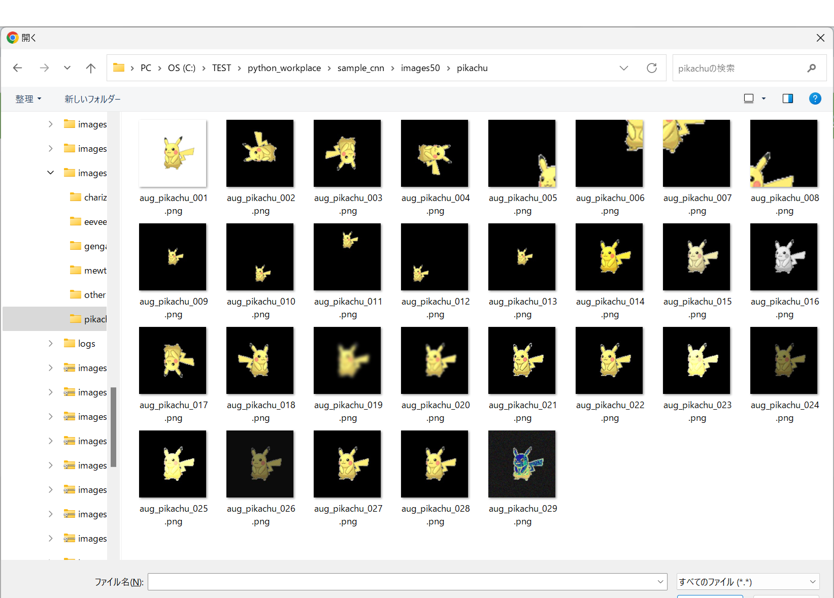
ポケモン809種の画像が120×120の形で保存されています。
VGG16を使用するにあたり、224×2224に加工し、データ拡張をしています。

pokemon-apiを使おうか検討しましたが、
最後に公開できないことを知り、諦めました。

今回試してみた内容

今回はWEBアプリで画像を投稿したら、その画像がどの様な分類になるか？
というものを作成したいと思います。

教師あり学習の中にある「分類（カテゴリ分け）」と「回帰（予測）」のうちの
「分類（カテゴリ分け）」にあたる画像分類を、CNNでVGG16を使って強化してやっていこうと思います。

※画像分類はCNNが得意だといわれています。

CNNってなにそれおいしいの？

ユースケースを考えてみました。
例えばGoogle Street Viewの画像として取り込んで学習させることで
画像がどこで写されたものか判別できるかもしれません。
目指せ迷子撲滅！
AirTagの位置の特定より正確な位置特定が出来る様になる未来が来るかも知れません。
また、テレビの生放送で自動的に位置情報が映像に出力されるかも知れません。

CNNとは？

畳み込みニューラルネットワーク（Convolutional Neural Network）
畳み込み層とプーリング層を重ね合わせて安定性を増していく取り組みです。
畳み込み層は、モデル内部でカーネルと同じ様な形状のデータを検知する層を畳み込み層といいます。
プーリング層は、データ誤差に対する特徴抽出の安定性を向上させる層です。
maxプーリングやaverageプーリングなどがあります。

VGG16とは？

Oxford大学のVisual Geometry Group（VGG）によって開発された深層学習モデルで、2014年のILSVRCコンペティションで高い評価を受けました。このモデルは、16の層から成り立っており、3×3の小さなフィルタを使用した畳み込み層が特徴です。

結論から行くと・・・

WEBまで作成できました。
ただ、flaskとかいろいろ本題から外れてしまうのでWEBに組み込む部分は割愛します。

初期画面

画像を選択し

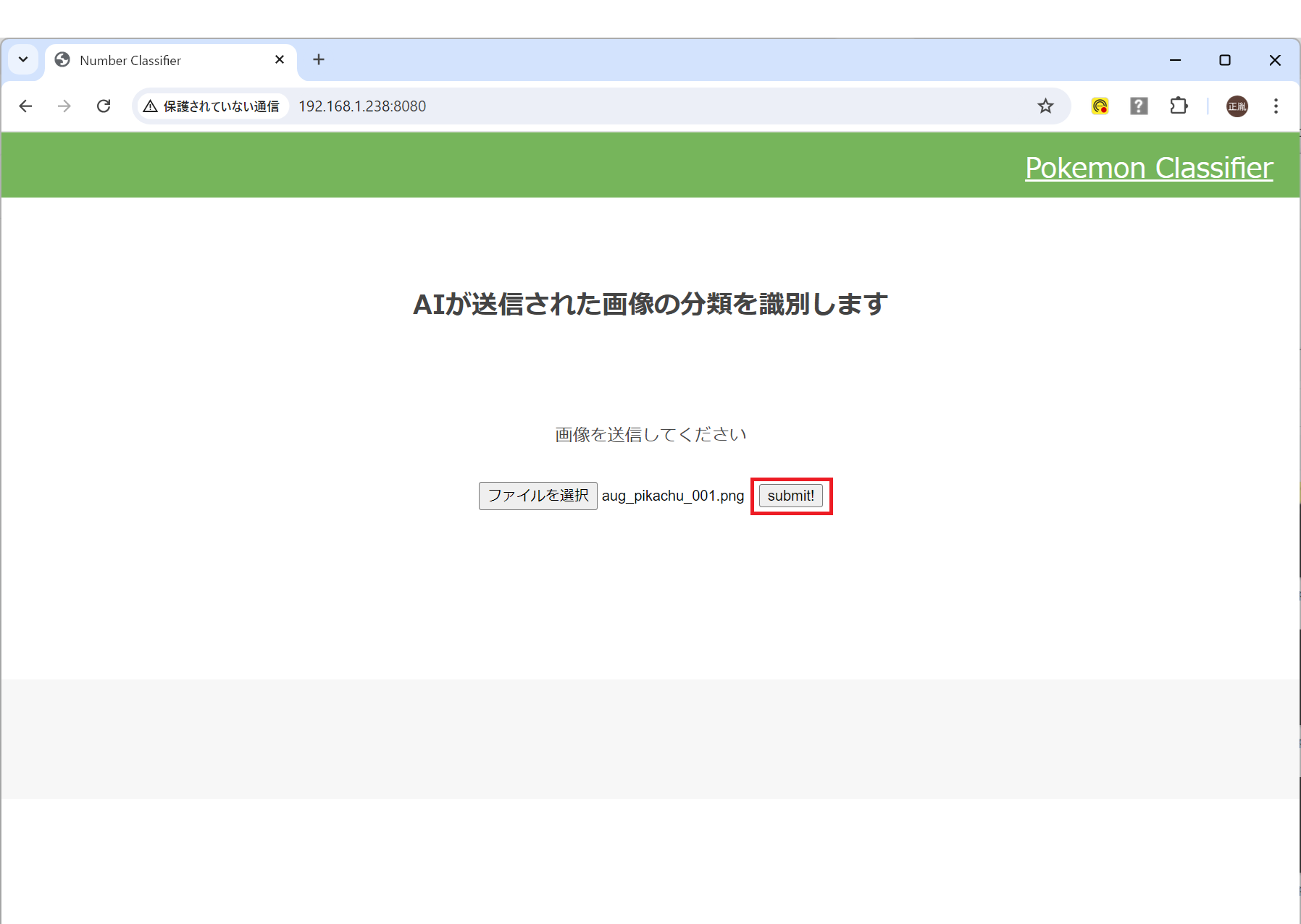
分類！

無事に分類できました。

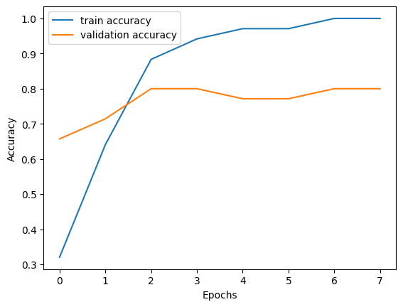
学習曲線は？

訓練データの学習率と、テストデータによる汎化性能を可視化したものです。
先ほども書きましたが、１画像につき約30種のデータ拡張を行ったとしても、訓練データが6割18枚、検証6枚、テスト6枚という事なので、次はデータをもっと大量に用意しようと思います。

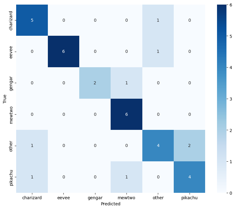
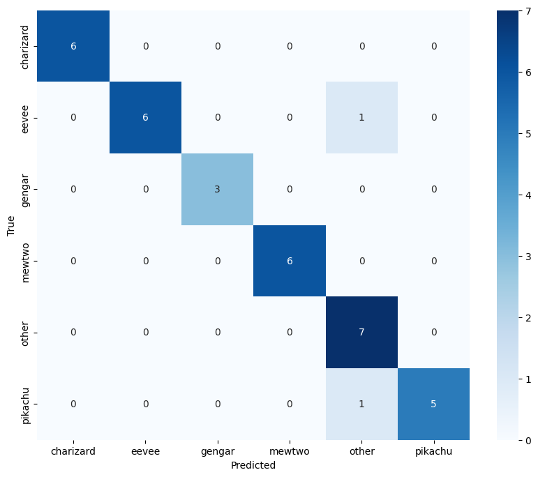
混同行列は？

どのクラス分類が予測としてどのクラス分類に判定されたかを可視化したものになります
左上から右下へ収束していると性能が良いと判断できるものです。
gengerのクラス分類が思わしくないので次の課題としてもう少し精度を上げていきたいです。

性能評価は？

クラス	精度 (precision)	再現率 (recall)	F1スコア (f1-score)	サポート (support)
charizard	0.75	0.50	0.60	6
eevee	0.75	0.86	0.80	7
gengar	1.00	0.67	0.80	3
mewtwo	0.55	1.00	0.71	6
other	0.67	0.57	0.62	7
pikachu	1.00	0.67	0.80	6
全体精度	0.71	35
平均値	0.79	0.71	0.72	35
加重平均	0.76	0.71	0.71	35

考察

課題として、もっと精度があげられるのではないかと考えています。

■前処理
画像をデータ拡張する数が非常に重要です。
訓練／検証／テストで６／２／２の割合にし、性能を評価していきます。

２０％しかテストできないので、テストデータが１枚適合しないだけでN％単位で
精度が落ちることを念頭に置く必要があります。

データ拡張の種類でやったこと
回転３種（90度、180度、270度）
拡大＋クロップ4種（縦横2倍に拡大後四隅を切り抜く）
縮小＋余白追加（縮小後が四隅になる様に余白を追加）
垂直変換
水平変換
彩度の強調／減衰
グレースケール
ぼかし２種
シャープネスの強調／減衰をそれぞれ変換２種
明るさ２種
ランダムなノイズ追加

■ハイパーパラメータの調整で試したこと
初期学習率、ドロップアウト率、エポック数、バッチサイズ（フィルター数）

■困ったこと
分類するクラスが多すぎると、GoogleColaboratoryのGPUのメモリが振り切れて実行できませんでした。
体感２万枚程度ならモデル作るぐらいはできそうです。
ただし、GridSearchするとかなりシビアで200枚の画像ぐらいでメモリが振り切れそうになりました。

後日談

無事に90%を超えることが出来ました。
理解しやすくするために層を減らしていましたが、増やしたところ精度が出ました。

差分のソース

    # 新しいCONV2D層とプーリング層を追加
    x = Conv2D(64, (3, 3), activation='relu', padding='same')(x)
    x = Conv2D(128, (3, 3), activation='relu', padding='same')(x)
    x = MaxPooling2D(pool_size=(2, 2))(x)
    x = Conv2D(256, (3, 3), activation='relu', padding='same')(x)
    x = Conv2D(512, (3, 3), activation='relu', padding='same')(x)
    x = MaxPooling2D(pool_size=(2, 2))(x)

学習曲線（後日談）

混同行列（後日談）

性能評価（後日談）

クラス	精度 (precision)	再現率 (recall)	F1スコア (f1-score)	サポート (support)
charizard	1.00	1.00	1.00	6
eevee	1.00	0.86	0.92	7
gengar	1.00	1.00	1.00	3
mewtwo	1.00	1.00	1.00	6
other	0.78	1.00	0.88	7
pikachu	1.00	0.83	0.91	6
accuracy			0.94	35
macro avg	0.96	0.95	0.95	35
weighted avg	0.96	0.94	0.94	35

今回使用した環境

WIndows11とGoogoleColaboratoryで実行しています。
やってる人にはおなじみだと思います。

!pip install tensorflow
!pip install scikit-learn
!pip install matplotlib
!pip install seaborn
!pip install scikeras

前処理をlocal PCで行い、
GoogleDriveに上げてZipエクストラクターで解凍
GoogleColaboratoryを使ってGPUを使って学習させていきました。

モデル作成のコード

import scikeras
from scikeras.wrappers import KerasClassifier
import tensorflow as tf
from tensorflow.keras.preprocessing.image import ImageDataGenerator
from tensorflow.keras.models import Model
from tensorflow.keras.layers import Flatten, Dense, Dropout, Input
from tensorflow.keras.optimizers import Adam
from tensorflow.keras.applications import VGG16
from tensorflow.keras.callbacks import EarlyStopping
from sklearn.model_selection import train_test_split
from sklearn.metrics import confusion_matrix,classification_report
import matplotlib.pyplot as plt
import seaborn as sns
import numpy as np

from google.colab import drive
import time

# タイムスタンプの表示
start_time = time.time()
print("開始時刻:", time.strftime("%Y-%m-%d %H:%M:%S", time.localtime(start_time)))

# ディレクトリの設定
drive.mount('/content/drive')

# データの準備
data_dir = '/content/drive/MyDrive/sample_cnn/images50'
datagen = ImageDataGenerator(rescale=1./255)
generator = datagen.flow_from_directory(
    data_dir,
    target_size=(224, 224),
    batch_size=32,
    class_mode='categorical',
    seed=42,
    shuffle=True
)

X, y = [], []
for _ in range(len(generator)):
    X_batch, y_batch = next(generator)
    X.append(X_batch)
    y.append(y_batch)

X = np.concatenate(X)
y = np.concatenate(y)

# クラスインデックスの確認
print(generator.class_indices)

# データを訓練、テストセットに分割
X_train, X_test, y_train, y_test = train_test_split(X, y, test_size=0.2, random_state=42)
X_train, X_val, y_train, y_val = train_test_split(X_train, y_train, test_size=0.25, random_state=42)

# クラスのサンプル数を確認
class_counts = np.bincount(y_train.argmax(axis=1))
print("Class counts in training data:", class_counts)

# モデルの構築
def create_model(learning_rate=0.0001, dropout_rate=0.5, dense_units=256, num_classes=6, **kwargs):
    base_model = VGG16(weights='imagenet', include_top=False, input_shape=(224, 224, 3))
    for layer in base_model.layers[:-4]:
        layer.trainable = False
    for layer in base_model.layers[-4:]:
        layer.trainable = True

    x = base_model.output
    x = Flatten()(x)
    x = Dense(dense_units, activation='relu')(x)
    x = Dropout(dropout_rate)(x)
    predictions = Dense(num_classes, activation='softmax')(x)

    model = Model(inputs=base_model.input, outputs=predictions)
    model.compile(optimizer=Adam(learning_rate=learning_rate),
                  loss='categorical_crossentropy',
                  metrics=['accuracy'])
    return model

# モデルの作成
model = create_model()

# EarlyStoppingの設定
early_stopping = EarlyStopping(monitor='val_loss', patience=5, restore_best_weights=True)

# モデルのトレーニング
history = model.fit(
    X_train,
    y_train,
    epochs=20,
    batch_size=32,
    validation_data=(X_val, y_val),
    callbacks=[early_stopping]
)

# テストデータでの評価
test_loss, test_accuracy = model.evaluate(X_test, y_test)
print(f"Test accuracy: {test_accuracy}")

# 学習曲線の表示
plt.plot(history.history['accuracy'], label='train accuracy')
plt.plot(history.history['val_accuracy'], label='validation accuracy')
plt.xlabel('Epochs')
plt.ylabel('Accuracy')
plt.legend()
plt.show()

# テストデータの予測
y_pred = model.predict(X_test)
y_pred_classes = np.argmax(y_pred, axis=1)
y_true = np.argmax(y_test, axis=1)

# 混同行列の計算
cm = confusion_matrix(y_true, y_pred_classes)

# クラスラベルの定義
class_names = list(generator.class_indices.keys())

# 混同行列のプロット
plt.figure(figsize=(10, 8))
sns.heatmap(cm, annot=True, fmt='d', cmap='Blues', xticklabels=class_names, yticklabels=class_names)
plt.xlabel('Predicted')
plt.ylabel('True')
plt.show()

# 性能評価のスコアを計算
report = classification_report(y_true, y_pred_classes, target_names=class_names)

# 性能評価のスコアを表示
print("分類レポート:\n", report)

# モデルの保存
model.save('/content/drive/MyDrive/model.h5')

# 終了時刻と実行時間の表示
end_time = time.time()
print("終了時刻:", time.strftime("%Y-%m-%d %H:%M:%S", time.localtime(end_time)))
print("実行時間:", end_time - start_time, "秒")

データ拡張のコード

import os
import shutil
from PIL import Image, ImageEnhance, ImageOps, ImageFilter
import numpy as np

# 変換関数の定義
def apply_transformations(image):
    # 画像をRGB形式に変換
    image = image.convert("RGB")
    
    # 画像を224×224にリサイズ
    image = image.resize((224, 224))
    
    transformations = [
        lambda x: x.rotate(90),
        lambda x: x.rotate(180),
        lambda x: x.rotate(270),
        lambda x: x.resize((448, 448)).crop((0, 0, 224, 224)),  # 拡大とクロップ（左上寄せ）
        lambda x: x.resize((448, 448)).crop((0, 224, 224, 448)),  # 拡大とクロップ（左下寄せ）
        lambda x: x.resize((448, 448)).crop((224, 224, 448, 448)),  # 拡大とクロップ（右下寄せ）
        lambda x: x.resize((448, 448)).crop((224, 0, 448, 224)),  # 拡大とクロップ（右上寄せ）
        lambda x: ImageOps.expand(x.resize((112, 112)), border=56, fill='black'),  # 縮小と余白の追加（左上寄せ）
        lambda x: ImageOps.expand(x.resize((112, 112)), border=(56, 112, 56, 0), fill='black'),  # 縮小と余白の追加（左下寄せ）
        lambda x: ImageOps.expand(x.resize((112, 112)), border=(56, 0, 56, 112), fill='black'),  # 縮小と余白の追加（右下寄せ）
        lambda x: ImageOps.expand(x.resize((112, 112)), border=(0, 112, 112, 0), fill='black'),  # 縮小と余白の追加（右上寄せ）
        lambda x: ImageOps.expand(x.resize((112, 112)), border=(56, 56, 56, 56), fill='black'),  # 縮小と余白の追加（上下中央）
        lambda x: ImageEnhance.Color(x).enhance(1.5),
        lambda x: ImageEnhance.Color(x).enhance(0.5),
        lambda x: x.convert("L"),
        lambda x: ImageOps.flip(x),
        lambda x: ImageOps.mirror(x),
        lambda x: x.filter(ImageFilter.GaussianBlur(5)),
        lambda x: x.filter(ImageFilter.GaussianBlur(2)),
        lambda x: x.filter(ImageFilter.UnsharpMask(2)),
        lambda x: x.filter(ImageFilter.UnsharpMask(1)),
        lambda x: ImageEnhance.Brightness(x).enhance(1.5),
        lambda x: ImageEnhance.Brightness(x).enhance(0.5),
        lambda x: ImageEnhance.Contrast(x).enhance(1.5),
        lambda x: ImageEnhance.Contrast(x).enhance(0.5),
        lambda x: ImageEnhance.Sharpness(x).enhance(2),
        lambda x: ImageEnhance.Sharpness(x).enhance(0.5),
        lambda x: Image.fromarray(np.array(x) + np.random.randint(0, 50, (x.height, x.width, 3), dtype='uint8'))  # ノイズ追加
    ]
    transformed_images = []
    for i, transformation in enumerate(transformations):
        transformed_image = transformation(image)
        transformed_images.append((transformed_image, f"aug_{i+1:03d}_"))
    return transformed_images

# ディレクトリの設定
source_dir = './images'
target_dir = './images50'

# 新しいディレクトリの作成
if not os.path.exists(target_dir):
    os.makedirs(target_dir)

# ポケモン名とディレクトリの対応
pokemon_dict = {
    "pikachu": "ピカチュウ",
    "charizard": "リザードン",
    "mewtwo": "ミュウツー",
    "eevee": "イーブイ",
    "gengar": "ゲンガー"
}

# 元データのコピーと分類
for filename in os.listdir(source_dir):
    if filename.endswith(('.png', '.jpg', '.jpeg')):
        name, ext = os.path.splitext(filename)
        if name in pokemon_dict:
            target_subdir = os.path.join(target_dir, name)
            if not os.path.exists(target_subdir):
                os.makedirs(target_subdir)
            target_path = os.path.join(target_subdir, f"aug_{name}_001{ext}")
            image = Image.open(os.path.join(source_dir, filename))
            image = image.resize((224, 224))  # 224×224にリサイズ
            image.save(target_path)

# `other` ディレクトリの作成
other_dir = os.path.join(target_dir, "other")
if not os.path.exists(other_dir):
    os.makedirs(other_dir)

# 変換データの生成と保存
for filename in os.listdir(source_dir):
    if filename.endswith(('.png', '.jpg', '.jpeg')):
        name, ext = os.path.splitext(filename)
        if name in pokemon_dict:
            image_path = os.path.join(source_dir, filename)
            image = Image.open(image_path)
            transformed_images = apply_transformations(image)
            for i, (transformed_image, prefix) in enumerate(transformed_images):
                new_filename = f"aug_{name}_{i+2:03d}{ext}"
                transformed_image.save(os.path.join(target_dir, name, new_filename))
        elif name == "snorlax":
            image_path = os.path.join(source_dir, filename)
            image = Image.open(image_path)
            transformed_images = apply_transformations(image)
            for i, (transformed_image, prefix) in enumerate(transformed_images):
                new_filename = f"aug_other_{i+2:03d}{ext}"
                transformed_image.save(os.path.join(other_dir, new_filename))

print("元データと変換データを含む新しいディレクトリが作成されました。")

モデル作成のコード（後日談のコード）

import scikeras
from scikeras.wrappers import KerasClassifier
import tensorflow as tf
from tensorflow.keras.preprocessing.image import ImageDataGenerator
from tensorflow.keras.models import Model
from tensorflow.keras.layers import Flatten, Dense, Dropout, Input,Conv2D, MaxPooling2D
from tensorflow.keras.optimizers import Adam
from tensorflow.keras.applications import VGG16
from tensorflow.keras.callbacks import EarlyStopping
from sklearn.model_selection import train_test_split
from sklearn.metrics import confusion_matrix,classification_report
import matplotlib.pyplot as plt
import seaborn as sns
import numpy as np

from google.colab import drive
import time

# タイムスタンプの表示
start_time = time.time()
print("開始時刻:", time.strftime("%Y-%m-%d %H:%M:%S", time.localtime(start_time)))

# ディレクトリの設定
drive.mount('/content/drive')

# データの準備
data_dir = '/content/drive/MyDrive/sample_cnn/images50'
datagen = ImageDataGenerator(rescale=1./255)
generator = datagen.flow_from_directory(
    data_dir,
    target_size=(224, 224),
    batch_size=32,
    class_mode='categorical',
    seed=42,
    shuffle=True
)

X, y = [], []
for _ in range(len(generator)):
    X_batch, y_batch = next(generator)
    X.append(X_batch)
    y.append(y_batch)

X = np.concatenate(X)
y = np.concatenate(y)

# クラスインデックスの確認
print(generator.class_indices)

# データを訓練、テストセットに分割
X_train, X_test, y_train, y_test = train_test_split(X, y, test_size=0.2, random_state=42)
X_train, X_val, y_train, y_val = train_test_split(X_train, y_train, test_size=0.25, random_state=42)

# クラスのサンプル数を確認
class_counts = np.bincount(y_train.argmax(axis=1))
print("Class counts in training data:", class_counts)

# モデルの構築
def create_model(learning_rate=0.0001, dropout_rate=0.5, dense_units=256, num_classes=6, **kwargs):
    base_model = VGG16(weights='imagenet', include_top=False, input_shape=(224, 224, 3))
    for layer in base_model.layers[:-4]:
        layer.trainable = False
    for layer in base_model.layers[-4:]:
        layer.trainable = True

    x = base_model.output

    # 新しいCONV2D層とプーリング層を追加
    x = Conv2D(64, (3, 3), activation='relu', padding='same')(x)
    x = Conv2D(128, (3, 3), activation='relu', padding='same')(x)
    x = MaxPooling2D(pool_size=(2, 2))(x)
    x = Conv2D(256, (3, 3), activation='relu', padding='same')(x)
    x = Conv2D(512, (3, 3), activation='relu', padding='same')(x)
    x = MaxPooling2D(pool_size=(2, 2))(x)

    x = Flatten()(x)
    x = Dense(dense_units, activation='relu')(x)
    x = Dropout(dropout_rate)(x)
    x = Dense(dense_units, activation='relu')(x)
    predictions = Dense(num_classes, activation='softmax')(x)

    model = Model(inputs=base_model.input, outputs=predictions)
    model.compile(optimizer=Adam(learning_rate=learning_rate),
                  loss='categorical_crossentropy',
                  metrics=['accuracy'])
    return model

# モデルの作成
model = create_model()

# EarlyStoppingの設定
early_stopping = EarlyStopping(monitor='val_loss', patience=5, restore_best_weights=True)

# モデルのトレーニング
history = model.fit(
    X_train,
    y_train,
    epochs=20,
    batch_size=32,
    validation_data=(X_val, y_val),
    callbacks=[early_stopping]
)

# テストデータでの評価
test_loss, test_accuracy = model.evaluate(X_test, y_test)
print(f"Test accuracy: {test_accuracy}")

# 学習曲線の表示
plt.plot(history.history['accuracy'], label='train accuracy')
plt.plot(history.history['val_accuracy'], label='validation accuracy')
plt.xlabel('Epochs')
plt.ylabel('Accuracy')
plt.legend()
plt.show()

# テストデータの予測
y_pred = model.predict(X_test)
y_pred_classes = np.argmax(y_pred, axis=1)
y_true = np.argmax(y_test, axis=1)

# 混同行列の計算
cm = confusion_matrix(y_true, y_pred_classes)

# クラスラベルの定義
class_names = list(generator.class_indices.keys())

# 混同行列のプロット
plt.figure(figsize=(10, 8))
sns.heatmap(cm, annot=True, fmt='d', cmap='Blues', xticklabels=class_names, yticklabels=class_names)
plt.xlabel('Predicted')
plt.ylabel('True')
plt.show()

# 性能評価のスコアを計算
report = classification_report(y_true, y_pred_classes, target_names=class_names)

# 性能評価のスコアを表示
print("分類レポート:\n", report)

# モデルの保存
model.save('/content/drive/MyDrive/model.h5')

# 終了時刻と実行時間の表示
end_time = time.time()
print("終了時刻:", time.strftime("%Y-%m-%d %H:%M:%S", time.localtime(end_time)))
print("実行時間:", end_time - start_time, "秒")

今回の手順

調べながらだったので、なかなかにごちゃごちゃしました。

・深層学習
・ハイパーパラメータチューニング
・VGG16の導入
・前処理の再加工
・ハイパーパラメータチューニング
・EarlyStoppingの導入
・前処理の再加工
・ハイパーパラメータチューニング
・前処理の再加工

一般的な手順

・前処理
・機械学習
・PoC
・深層学習
・ハイパーパラメータチューニング