はじめに

MICCAI(Medical Image Computing and Computer Assisted Intervention)2018から以下の論文のまとめ。

[1] Y. Chen, et. al."Efficient and Accurate MRI Super-Resolution using a Generative Adversarial Network and 3D Multi-Level Densely Connected Network"

著者らのgithubページはあるが
https://github.com/YuhuaBillChen/mDCSRN-MRI
コードそのものは見当たらず。

モデル名は mDCSRN (multi-level densely connected super-resolution networks)

概要

MRI画像を超解像するモデル
3Dの画像を入力とし、DenseNet（[2]）のアーキテクチャで超解像する
GANを用いた学習を行う

アーキテクチャ

アーキテクチャの概要図（[1]のfigure 1 より）

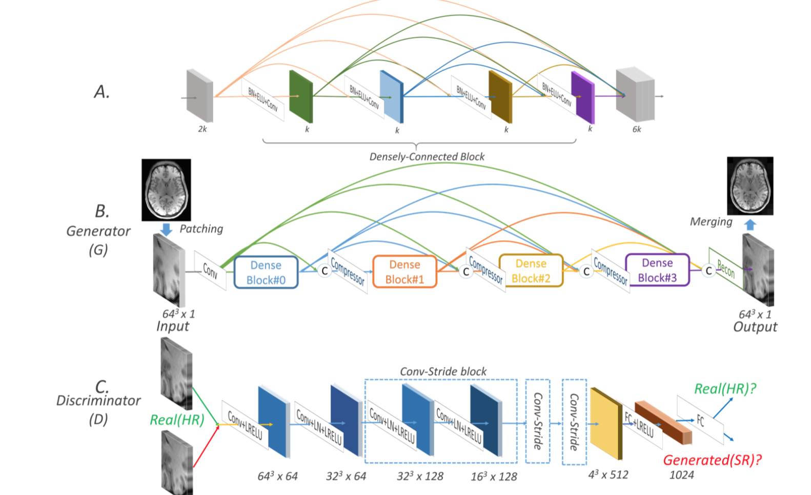
最上部 A は3DのDense block。

本 mDCSRN モデルのgeneratorはこれをさらに densely につなげている。（B)

一方で discriminator は、ほぼほぼ SRGAN（[3]）と同じだが、batch normをlayer normに変えている。

コスト関数

コスト関数は１）Wasserstein-GAN（[4]）のgradient penaltyしたものに、２）超解像した出力画像とground truthとのL1 loss、を加えたもの。

loss = loss_{int} + loss_{GAN}

$loss_{int}$ は

\begin{eqnarray}
loss_{int} &=& loss_{L1} \ / \ LHW \\
&=& \sum^L_{z=1} \sum^H_{y=1} \sum^W_{x=1} \  | \  I^{HR}_{x,y,z} - I^{SR}_{x,y,z} | \ / \ LHW \\
\end{eqnarray}

$loss_{GAN}$ は

\begin{eqnarray}
loss_{GAN} &=& loss_{WGAN, D} \\
&=& -D_{WGAN, \theta}(I^{SR})
\end{eqnarray}

ここで $I^{SR}$ はモデルで超解像した出力。 $I^{HR}$ はground truth。

入力画像の作り方

高解像な ground truth に対応する低解像な入力画像が必要となるが、これは[5]の手法を用いて生成する。

FFTで高解像度画像をk-spaceに変換する
3次元k-spaceの周囲をゼロにすることで解像度を下げる
FFT逆変換で画像に戻し、サイズが元に一致するよう線形に内挿する

実験の諸設定

データセット

こちら[6]から1,113データを集めた。

実験環境

フレームワーク：tensorflow
GPU：Nvidia GTX 1080Ti

学習の設定

最適化：Adam
batch size：2
step：500k（最初の10kはgeneratorのみでL1 lossで学習した後にdiscriminatorを加え、Dの学習７回につきGを１回学習させる。500回毎にはDのみ200回学習させる。）

比較モデル

FSRCNN、SRResNetなど。

本手法の異なる設定のモデル

denseNetの部分のunit数やblock数を変える
GANを用いる or 用いない

メトリクス

SSIM(subject-wise average structural similarity index)
PSNR(peak signal to noise ratio)
NRMSE(normalized root mean squared error)

結果

本手法でblock数とunit数を変えた比較

本手法 mDCSRN におけるblock数とunit数を変えた場合の性能、メモリ数、実行速度は以下。

block数2でunitは4の b2u4が速度が早くパラメータ数も少ないが、性能は b4u4がいい。

他のモデルとの比較

Bicubic interpolation、3D FSRCNN、3D SRResNetとの比較は以下。

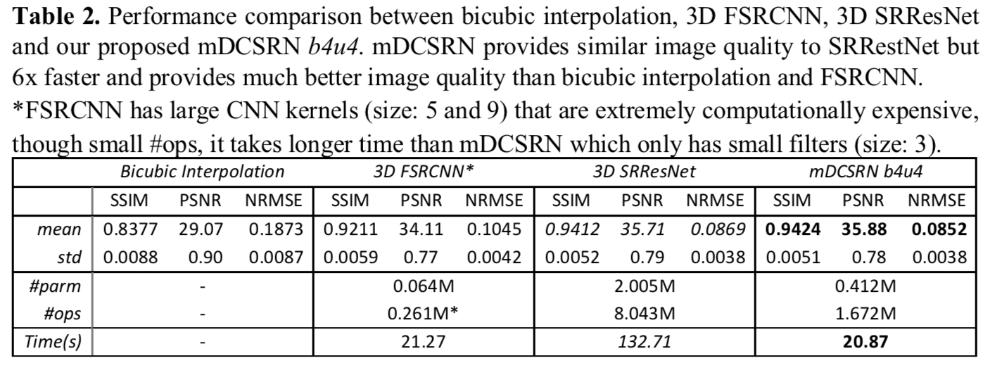
本手法が各メトリクスにおいて他の手法を上回っていて、かつ実行速度も早い。

他の手法との出力結果の比較

GANを加えるとhigh perceptualになっている。

結論

本手法 mDCSRN は（特にGAN lossを用いた mDCSRN-GANは）性能も他を上回り、かつ実行速度も上回った。

reference

[2] Huang, Gao, et al. "Densely connected convolutional networks." Proceedings of the IEEE conference on computer vision and pattern recognition. Vol. 1. No. 2. 2017.

[3] Ledig,Christian,etal."Photo-RealisticSingleImageSuper-ResolutionUsingaGenerative Adversarial Network." Proceedings of the IEEE Conference on Computer Vision and Pattern Recognition. 2017.

[4] Arjovsky, Martin, Soumith Chintala, and Léon Bottou. "Wasserstein gan." arXiv preprint arXiv:1701.07875 (2017).

[5] Chen, Yuhua, et al, "Brain MRI super resolution using 3D deep densely connected neural networks," Proceedings of 15th International Symposium on Biomedical Imaging (ISBI 2018), pp. 739-742.

[6] David C. Van Essen, Stephen M. Smith, Deanna M. Barch, Timothy E.J. Behrens, Essa Yacoub, Kamil Ugurbil, for the WU- Minn HCP Consortium. (2013). The WU-Minn Human Connectome Project: An overview. NeuroImage 80(2013):62-79.

論文まとめ：Efficient and Accurate MRI Super-Resolution using a Generative Adversarial Network and 3D Multi-Level Densely Connected Network