はじめに
現在開催中の NIPS2018 からnVIDIAの以下の論文
[1] T. Wang, et. al. "Video-to-Video Synthesis"
のまとめ
NIPSの該当ページ
https://nips.cc/Conferences/2018/Schedule?showEvent=11133
論文のリンク
http://papers.nips.cc/paper/7391-video-to-video-synthesis.pdf
Githubの公式コード
https://github.com/NVIDIA/vid2vid
デモビデオ
https://www.youtube.com/watch?v=5zlcXTCpQqM
このビデオを確認する限り、かなり精度よく生成されている
概要
- シーケンシャルな segmentation mask などから動画を生成するモデル
以下の[1]Figure 1 は生成した動画(の中の1フレーム)の例。
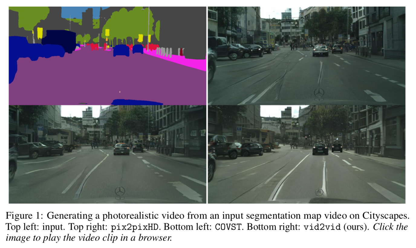
左上は segmentation mask、右上はpix2pixHDを使って生成した画像、左下はCOVSTを使って生成した画像、右下が本手法を使って生成した画像。
ざっと見、リアルでかつ、歪みが少ないハイクオリティな画像が生成されている。
アーキテクチャ
変数の定義
まず変数の定義。
$s _1^T ={ s _1, s _2, \cdots , s _T }$ :シーケンシャルなsegmentation mask
$x _1^T ={ x _1, x _2, \cdots , x _T }$ : $s _1^T$ に対応するシーケンシャルな動画のフレーム
$ \tilde{x} _1^T ={ \tilde{x} _1, \tilde{x} _2, \cdots , \tilde{x} _T }$ : $s _1^T$ から生成されるシーケンシャルな動画のフレーム
目的
次に目的。$s _1^T$ を入力した時にモデルが生成する動画 $\tilde{x} _1^T$ を実際の動画のようなリアルなものに近づけること。つまり
p(\tilde{x} _1^T | s _1^T) = p(x _1^T | s _1^T)
マルコフ性を仮定すると
p(\tilde{x} _1^T | s _1^T) = \prod ^T_{t=1} p(\tilde{x} _t | \tilde{x} _{t-L}^{t-1}, s ^t_{t-L} )
$t$ フレーム目の生成画像 $\tilde{x} _t$ は $L$ フレーム前から $1$ フレーム前までの生成画像 $\tilde{x} _{t-L}^{t-1} $ と現在(tフレーム)から $L$ フレーム前までのsegmentation mask $s ^t _{t-L}$ で決まる。
ネットワーク
この条件付き確率 $p(\tilde{x} _t | \tilde{x} _{t-L} ^{t-1}, s ^t _{t-L} )$ を
\tilde{x} _t = F(\tilde{x} _{t-L} ^{t-1} , s^t_{t-L})
としてモデル化する。つまりネットワークに入力する1つは $s ^t _{t-L}$ で、もう1つは $\tilde{x} _{t-L} ^{t-1}$ 。
これにより $\tilde{x} _t$ が出力される。これを繰り返すことで次々と $\tilde{x} _t$ が生み出される。
$F$ は具体的に以下のようにする。
\begin{equation}
F(\tilde{x} _{t-L} ^{t-1} , s^t_{t-L}) = (1 - \tilde{m} _t ) \odot  \tilde{w} _{t-1} (\tilde{x} _{t-1} ) + \tilde{m} _t \odot \tilde{h} _t
\end{equation}
$\odot$ はアダマール積。
まず $\tilde{w} _{t-1} = W (\tilde{x} _{t-L} ^{t-1} , s^t _{t-L})$ は $\tilde{x} _{t-1}$ から $\tilde{x} _{t}$ へ変換する optical flow。
$\tilde{h} _t = H(\tilde{x} _{t-L} ^{t-1} , s^t _{t-L})$ はgeneratorから生成される hallucinated (幻覚と訳すべき??)な画像。これは optical flowでは対応できない occulusionな部分で使用する。
$\tilde{m} _t = M(\tilde{x} _{t-L} ^{t-1} , s^t _{t-L})$ はocculusion mask。0, 1のバイナリーではなく、0から1の連続変数。
つまり、右辺第1項で optical flow から画像を生成し、第2項で optical flowでは生成できない occulusion の部分の画像を生成する。
これをネットワークの図で見ると、コアな部分は下図 [1]Figure 8 の $G_1$ ようになる。
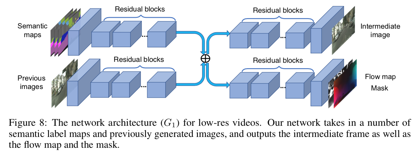
左上から $s^t _{t-L}$ を入力し、左下から $\tilde{x} _{t-L} ^{t-1}$ を入力する。
これに対して右上から hallucinated な画像 $\tilde{h} _t$ を生成し、右下から optical flow $\tilde{w} _{t}$ と occulusion mask $\tilde{m} _t$ を出力している。
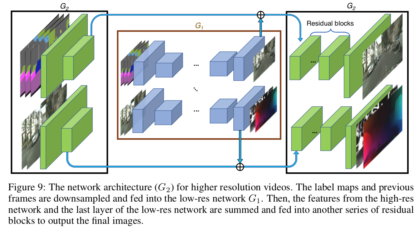
超解像な画像生成
上記の $G_1$ を鮮明にするため、下図[1]Figure 9 のような $G_2$ を加える。
Discriminator
Discriminator は2種類。
1つ目は画像とsegmentation maskのペアが生成されたもの $( \tilde{x} _t, x _t )$ か、リアルなペア $(x _t, s _t)$ かを判定する $D _I$。これにより生成される画像がリアルな画像に近づく。
2つ目はシーケンシャルな画像とそれに対応する optical flow が原動画とoptical flowのペア $(x ^{t-1} _{t-K}, w ^{t-2} _{t-K})$ か、あるいは生成された動画と optical flowのペア $( \tilde{x} ^{t-1} _{t-K}, w ^{t-2} _{t-K})$ かを判定する $D _V$ 。これにより動画が滑らかなものになる。
目的関数
目的関数全体は以下。
\begin{equation}
\min_F (\max_{D_I} \mathcal{L} _I (F,D_I) + \max _{D_V} \mathcal{L}_V (F,D_V)) + \lambda_W \mathcal{L}_W(F)
\end{equation}
$\mathcal{L} _I$ は $D _I$ に関わるadversarial なロス、$\mathcal{L} _V$ は $D _V$ に関わる adverarial なロス、$\mathcal{L} _W$ は optical flow に関わるロス。
画像のリアルさを判定するロス
画像のリアルさを判定する adversarial なロス $\mathcal{L} _I$ は以下。
\begin{equation}
\mathcal{L} _I = E_{\phi _I (x_1^T, s_1^T)} [\log D_I (x_i, s_i)] + E_{\phi _I (\tilde{x}_1^T, s_1^T)} [\log (1 -D_I (\tilde{x}_i, s_i))]
\end{equation}
ビデオのリアルさを判定するロス
ビデオのリアルさを判定する adversarial なロスは以下。
\begin{equation}
\mathcal{L} _V = E_{\phi _V (w_1^{T-1} ,x_1^T, s_1^T)} [\log D_V (x^{i-1}_{i-K}, w_{i-K}^{i-2})] + E_{\phi _V (w_1^{T-1} ,\tilde{x}_1^T, s_1^T)} [\log (1 - D_V (\tilde{x}^{i-1}_{i-K}, w_{i-K}^{i-2}))]
\end{equation}
optical flow をそれらしくするロス
$\mathcal{L} _W$ では optical flow の推定値を実動画のそれに近づけるため以下とする。
\begin{equation}
\mathcal{L} _W = \frac{1}{T-1} \sum ^{T-1}_{t=1} (\| \tilde{w}_t - w_t \| _1 + \| \tilde{w}_t (x_t) - x_{t-1} \| _1)
\end{equation}
右辺第1項で実動画の optical flow と 推定された optical flow との差をとっている。
右辺第2項で推定された optical flow によって実動画の次フレームを予測した値 $\tilde{w} _t (x _t)$ と実動画の実際の次フレーム $x _{t-1}$ との差をとっている。
実験と結果
Cityscapes dataset で他のモデルと比較した結果は以下。
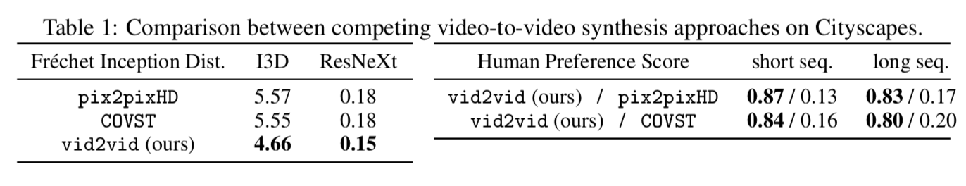
左側がFrechet Inception Distanceによる評価、右側が人のpreference score。
pix2pix及びCOVSTと比較したところ、いずれの評価手法においても最も評価が高い。
書きかけ