1. モチベーション
R interface to Kerasに従って、RでKerasを試してみます。今回は、インストールと手書き文字分類までの流れをメモしておきます。※GPUバージョンの構築は失敗したので、またそのうち追記します。(OS: Windows7)
2. Rtoolsのインストール
R interface to Kerasの手順の通りに進めていくと、Rtools3.4が必要というエラーが出ることがあります。そこで、まず初めに最新のRtoolsをインストールしておきます。
Rtoolsのサイトからダウンロードして、手順に従ってインストールします。
よく読みませんでしたが、チェックボックスはすべてチェックしました。
3. Python 3.5のインストール
Python3.5がインストールされていないと、以下のエラーメッセージが出ます。
Errorython: Installing TensorFlow requires a 64-bit version of Python 3.5 Please install 64-bit Python 3.5 to continue, supported versions include: - Anaconda Python (Recommended): https://www.continuum.io/downloads#windows - Python Software Foundation : https://www.python.org/downloads/release/python-353/ Note that if you install from Python Software Foundation you must install exactly Python 3.5 (as opposed to 3.6 or higher).
というわけで、レコメンドされた通り、Anacondaを利用します。
ここまで終われば、普通に進められます。
4. Kerasパッケージのインストール
R interface to Kerasの通り、devtoolsでGithubからkerasパッケージをインストールします。(ついでに、tensolflowパッケージも新しいのを入れておきます。)
devtools::install_github("rstudio/keras")
devtools::install_github("rstudio/tensorflow")
5. TensorFlowのインストール
kerasを読み込み、install_tensorflow()関数を利用してTensorFlowをインストールします。
CPUを使う場合は以下の通りです。
library(keras)
install_tensorflow()
GPUを使いたい場合は、Installing the GPU Versionを参考にして、CUDA ToolkitとcuDNNをインストールします。cuDNNは、ダウンロードしたzipファイルを解凍後、環境変数に\binへのPathを追加します。
それから、以下の通りTensorFlowをインストールします。
library(keras)
install_tensorflow(gpu = TRUE)
※GPU版のインストールはできたのですが、dataset_mnist()を実行したところ、以下のエラーが出てしまったので、今回はCPUバージョンでチュートリアルを行います。
Error: Python module tensorflow.contrib.keras.python.keras was not found.
6. チュートリアル(MNISTデータのDNN)
mnist_mlp.Rに従って、有名なMNISTデータの分類を試してみます。
dataset_minist()関数でデータセットをロードできます。
他のデータセットです。
| 関数名 | データの内容 |
|---|---|
| dataset_boston_housing | Boston housing price regression dataset |
| dataset_cifar10 | CIFAR10 small image classification |
| dataset_cifar100 | CIFAR100 small image classification |
| dataset_imdb | IMDB Movie reviews sentiment classification |
| dataset_mnist | MNIST database of handwritten digits |
| dataset_reuters | Reuters newswire topics classification |
| dataset_reuters_word_index | Reuters newswire topics classification |
6-1. データの準備
MNISTデータは、train(学習データ)とtest(テストデータ)を含むリスト形式になっており、それぞれ、説明変数をx、目的変数をyとした配列を持っています。
library(keras)
mnist <- dataset_mnist()

# 学習データ
x_train <- mnist$train$x #説明変数
y_train <- mnist$train$y #目的変数

# テストデータ
x_test <- mnist$test$x #説明変数
y_test <- mnist$test$y #目的変数
説明変数データを以下の通り変換します。
x_train <- array(as.numeric(x_train), dim = c(dim(x_train)[[1]], 784))
x_test <- array(as.numeric(x_test), dim = c(dim(x_test)[[1]], 784))
学習データは、60000行、784列(28 x 28)というmatrixになります。
また、テストデータは、10000行、784列(28 x 28)というmatrixになります。
各値は、0-255の値となっていますが、これを規格化しておきます。
x_train <- x_train / 255
x_test <- x_test / 255
目的変数の方は、0-9の数字(Integer形式)になっています。
これを0、1の値を持つマトリックスに変換しておきます。
例えば、値が9であれば、1から9列目が0で、10列目が1となるようなマトリックスです。
num_classes <- 10
y_train <- to_categorical(y_train, num_classes)
y_test <- to_categorical(y_test, num_classes)
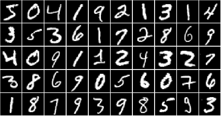
6-2. 視覚化
手書き文字(説明変数)を視覚化してみます。今回は以下の関数を作ります。
view_MNIST <- function(data=x_train, range=1:50, row=5, col=10){
  par(mfrow=c(row,col))
  par(mar=c(0.1,0.1,0.1,0.1))
  for(i in range){
    m <- matrix(data[i,], 28,28)
    image(t(m[28:1,]), col=gray(0:255/255), axes=F)
  }
}
以下のように使います。今回は学習データの50枚目までを、5行10列で表示します。
view_MNIST(data=x_train, range=1:50, row=5, col=10)
6-3. モデリング
チュートリアルのまま、多層パーセプトロンのモデルオブジェクトを作成します。
入力は、28 x 28 = 784個なので、input_shape=c(784)と指定します。
model <- keras_model_sequential()
model %>%
  layer_dense(units = 256, activation = 'relu', input_shape = c(784)) %>%
  layer_dropout(rate = 0.4) %>%
  layer_dense(units = 128, activation = 'relu') %>%
  layer_dropout(rate = 0.3) %>%
  layer_dense(units = 10, activation = 'softmax')
モデルの構成は、summary()関数で確認できます。
summary(model)

6-4. コンパイルとフィッティング
続いて、最適化の際の評価手法などを指定してコンパイルします。
model %>% compile(
  loss = 'categorical_crossentropy',
  optimizer = optimizer_rmsprop(),
  metrics = c('accuracy')
)
フィッティングは以下の通りです。
batch_size = 128
epochs = 30

history <- model %>% fit(
  x_train, y_train,
  batch_size = batch_size,
  epochs = epochs,
  verbose = 1,
  callbacks = callback_tensorboard(log_dir = "logs/run_b"),
  validation_split = 0.2
)
plot()を使うと、lossとmetrics_accuracyのプロットを見ることができます。
plot(history)

6-5. 評価
evaluate()関数で精度を確認できます。
score <- model %>% evaluate(
  x_test, y_test,
  verbose = 0
)

score
> score
[[1]]
[1] 0.1184483 #loss

[[2]]
[1] 0.9804 #精度
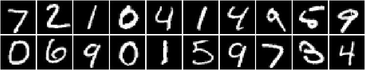
6-6. 予測結果
結果は、いつも通り、predict()で得られます。
classes <- model %>% predict(x_test, batch_size = 128)
round(classes)

# 1列目が0、10列目が9
>round(classes[1:20,])
         [,1] [,2] [,3] [,4] [,5] [,6] [,7] [,8] [,9] [,10]
    [1,]    0    0    0    0    0    0    0    1    0     0
    [2,]    0    0    1    0    0    0    0    0    0     0
    [3,]    0    1    0    0    0    0    0    0    0     0
    [4,]    1    0    0    0    0    0    0    0    0     0
    [5,]    0    0    0    0    1    0    0    0    0     0
    [6,]    0    1    0    0    0    0    0    0    0     0
    [7,]    0    0    0    0    1    0    0    0    0     0
    [8,]    0    0    0    0    0    0    0    0    0     1
    [9,]    0    0    0    0    0    1    0    0    0     0
   [10,]    0    0    0    0    0    0    0    0    0     1
   [11,]    1    0    0    0    0    0    0    0    0     0
   [12,]    0    0    0    0    0    0    1    0    0     0
   [13,]    0    0    0    0    0    0    0    0    0     1
   [14,]    1    0    0    0    0    0    0    0    0     0
   [15,]    0    1    0    0    0    0    0    0    0     0
   [16,]    0    0    0    0    0    1    0    0    0     0
   [17,]    0    0    0    0    0    0    0    0    0     1
   [18,]    0    0    0    0    0    0    0    1    0     0
   [19,]    0    0    0    1    0    0    0    0    0     0
   [20,]    0    0    0    0    1    0    0    0    0     0


# 実際のテストデータ
view_MNIST(data=x_test, 1:20)