1. Summary
本記事では,Hasitie,Tibshirani,Friedman(2009).The elements of statistical learningのchapter 4 Linear Methods for Classificationのロジスティック回帰分析について書いてある部分(や書いてない部分,自分の印象)についてまとめ,パラメータ推定のサンプルコードを添付しました.
2. What is logistic regression?
データ分析の目的の一つにクラス判別があります.クラス判別というのは,観察や実験によって得られた個体のデータから,個体がどのグループ(=クラス)に属するかを判定することを指します.ロジスティック回帰分析では,「ある個体xが観測された場合,その個体がどのグループに属するかの確率」,つまり,$P(G=k|X=x),(k=1,\cdots,K)$という事後確率をモデル化することを目的とします.事後確率は確率なので全てを足して1にならなければなりません.個体xが観測されたとして,それぞれのグループに属する事後確率は
\begin{eqnarray}
P(G=k|X=x) &=& \frac{\exp(a_{k0}+\beta_k^Tx)}{1+\sum_{l=1}^{K-1}\exp(a_{l0}+\beta_l^Tx)}\ (k=1,\cdots,K-1)\\
P(G=K|X=x) &=& \frac{1}{1+\sum_{l=1}^{K-1}\exp(a_{l0}+\beta_l^Tx)}
\end{eqnarray}
のように表されます.簡単な計算で$\sum_{k}P(G=k|X=x)=1$(全確率=1)であることがわかります.$K=2$(2クラス判別)の場合は単純に
\begin{eqnarray}
P(G=1|X=x) &=& \frac{\exp(a_{k0}+\beta_k^Tx)}{1+\exp(a_{10}+\beta_1^Tx)}\\
P(G=2|X=x) &=& \frac{1}{1+\exp(a_{10}+\beta_1^Tx)}
\end{eqnarray}
となります.以下に$K=2$として,$a,b$を変化させたロジスティック関数$P(G=1|X=x)$のグラフを示します.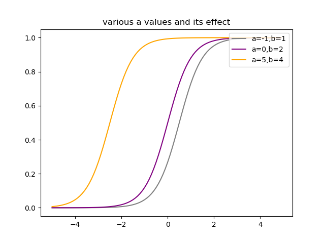
$a$を変化させると,曲線の形はそのままに,左右方向にシフトしている様子がわかります.このことから,$a$はロジスティック関数の位置を決めているパラメータといえるでしょう.
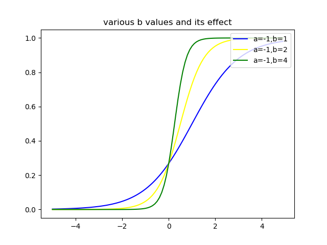 次に$b$を変化させると,曲線の曲がり方が変化するということがわかります.このことから,$b$はロジスティック関数の曲率を決めるパラメータといえるでしょう.以上のグラフでは,$b,x$はスカラーとしましたが,ベクトルの場合も同様の議論ができます.項目反応理論(Item Response Theory,IRT)はこのロジスティック関数を基にした理論で,学力を測ることなどに利用されているようです(詳しくはあまり知らないので勉強します).
item response theory (IRT) (also known as latent trait theory, strong true score theory, or modern mental test theory) is a paradigm for the design, analysis, and scoring of tests, questionnaires, and similar instruments measuring abilities, attitudes, or other variables. It is a theory of testing based on the relationship between individuals' performances on a test item and the test takers' levels of performance on an overall measure of the ability that item was designed to measure. (wikipedia (Item response theory)),(日本語ver.はこちら)
(どうやらテストや質問紙の項目に対する反応から受験者の性質や,テストや質問紙の項目の難易度や識別力を測定し,デザインするための理論らしい.)
通常のロジスティック回帰によるクラス判別では,計算された$P(G=k|X=x)$のうち,最も事後確率が大きいクラスに個体xが属するというように判断します.ロジスティック回帰のパラメータ推定について考えます.
3. How to estimate parameters
ロジスティック回帰のパラメータはXが与えられた下でのGの条件付き確率$P(G|X)$を用いて最尤法によって推定されます.多クラス分類の場合,事後確率が多項分布に従うと考えると,N個の個体xが観測された際の対数尤度は,$p_k(x_i;\theta)=P(G=k|X=x_i;\theta)$とすると,
\begin{eqnarray}
l(\theta) &=& \log\prod_{i=1}^Np_{g_i}(x_i;\theta)\\
&=& \sum_{i=1}^N\log p_{g_i}(x_i;\theta)\ (k=1,\cdots,K)
\end{eqnarray}
となります.議論を単純にするため(←The elements of statistical learningにもこう書いてます!),以下では2クラス分類問題のパラメータ推定について考えます.2クラス分類では$y_i$,$p_i$を以下のように定めると便利です.
\begin{eqnarray}
y_i &=& \left\{
\begin{array}{l}
1\ if\ g_i=1\\
0\ if\ g_i=2
\end{array}\right.\\\\
p_i(x;\theta) &=& \left\{
\begin{array}{l}
p(x;\theta)\ \ (if\ i=1)\\
1-p(x;\theta)\ \ (if\ i=2)
\end{array}\right.
\end{eqnarray}
以上のように定めた場合,事後確率は二項分布$Bin(1,p(x_i;\theta))$に従うため,対数尤度は以下のように表せます.
\begin{eqnarray}
l(\beta) &=& \log\prod_{i=1}^Np(x_i;\theta)^{y_i}(1-p(x_i;\theta))^{1-y_i}\\
&=& \sum_{i=1}^N\{y_i\log p(x_i;\theta)+(1-y_i)\log (1-p(x_i;\theta))\}\\
&=& \sum_{i=1}^N\{y_i\log \frac{\exp(\beta^Tx_i)}{1+\exp(\beta^Tx_i)}+(1-y_i)\log \frac{1}{1+\exp(\beta^Tx_i)}\}\\
&=& \sum_{i=1}^N\{y_i[\log\exp(\beta^Tx_i)-\log(1+\exp(\beta^Tx_i))]+(1-y_i)[\log 1-\log(1+\exp(\beta^Tx_i))]\}\\
&=& \sum_{i=1}^N\{y_i\beta^Tx_i-\log(1+\exp(\beta^Tx_i))\}\\
\end{eqnarray}
ここで$x_i$は切片項のために$x_i=(1,x_{i1},\cdots,x_{ip})^T$となっており,$\beta$も切片を含んで$\beta = (\beta_{10},\beta_1)$となっています.対数尤度を最大化するために,1次の偏微分を0とおきます.
\begin{eqnarray}
\frac{\partial l(\beta)}{\partial \beta}&=&\sum_{i=1}^N(y_ix_i-\frac{\exp(\beta^Tx_i)}{1+\exp(\beta^Tx_i)}x_i)\\
&=& \sum_{i=1}^N(y_i-p(x_i;\beta))x_i = 0\\
&\Leftrightarrow&\sum_{i=1}^Ny_ix_i = \sum_{i=1}^Np(x_i;\beta)x_i\\
\end{eqnarray}
以上の変形から分かるように,1次の偏微分を0とおいた解は$p+1$の$\beta$に関する非線形方程式となっています.しかし,$x_i$の第1成分が全て1であることに注意すると,最初の方程式は$\sum_{i=1}^Ny_i=\sum_{i=1}^Np(x_i;\beta)$となることがわかり,これはクラス1の期待度数が観測数と一致するということを表しています.この非線形方程式を解くために,二階の偏微分もしくは,ヘッセ行列を用いるNewton-Raphson法を利用します.この対数尤度に対する二回の偏微分は
\begin{eqnarray}
\frac{\partial^2 l(\beta)}{\partial \beta\partial\beta^T} &=& \frac{\partial}{\partial\beta^T}\sum_{i=1}^N(y_i-\frac{\exp(\beta^Tx_i)}{1+\exp(\beta^Tx_i)})x_i\\
&=&-\sum_{i=1}^N[\frac{e^{\beta^Tx_i}x_ix_i^T(1+\exp(\beta^Tx_i))-e^{\beta^Tx_i}x_i\exp(\beta^Tx_i)x_i^T}{(1+\exp(\beta^Tx_i))^2}]\\
&=&-\sum_{i=1}^N[\frac{e^{\beta^Tx_i}x_ix_i^T+\exp^{2\beta^Tx_i}x_ix_i^T-e^{2\beta^Tx_i}x_ix_i^T}{(1+\exp(\beta^Tx_i))^2}]\\
&=&-\sum_{i=1}^N\frac{e^{\beta^Tx_i}}{(1+\exp(\beta^Tx_i))^2}x_ix_i^T\\
&=&-\sum_{i=1}^N\frac{e^{\beta^Tx_i}}{1+\exp(\beta^Tx_i)}\frac{1}{1+\exp(\beta^Tx_i)}x_ix_i^T\\
&=&-\sum_{i=1}^Np(x_i;\beta)(1-p(x_i;\beta))x_ix_i^T
\end{eqnarray}
となります.現在の係数の推定値を$\beta^{old}$とすると,Newton-Raphson法での更新式は,
\beta^{new} = \beta^{old}-\biggl(\frac{\partial^2 l(\beta)}{\partial \beta\partial\beta^T}\biggr)^{-1}\frac{\partial l(\beta)}{\partial \beta}
で与えられます.これらを行列形式で書くと,
\begin{eqnarray}
\frac{\partial l(\beta)}{\partial \beta}&=&X^T(y-p)\\
\frac{\partial^2 l(\beta)}{\partial \beta\partial\beta^T}&=&-X^TWX
\end{eqnarray}
で表されます.ここで,$y,p$は$y=(y_1,\cdots,y_N)^T$,$p=(p(x_1;\beta^{old}),\cdots,p(x_N;\beta^{old}))^T$とし,$W$は$p(x_i;\beta)(1-p(x_i;\beta))$をi番目の対角成分に持つ対角行列としています.行列表現によるNewton-Raphson法の更新式は
\begin{eqnarray}
\beta^{new} &=& \beta^{old} + (X^TWX)^{-1}X^T(y-p)\\
&=& (X^TWX)^{-1}(X^TWX\beta^{old}+X^T(y-p))\\
&=& (X^TWX)^{-1}X^TW(X\beta^{old}+W^{-1}(y-p))\\
&=& (X^TWX)^{-1}X^TWz\\
&&(z:=X\beta^{old}+W^{-1}(y-p)\mbox{と置いた})
\end{eqnarray}
と書き表すことができます.これは以下の重み付き交互最小二乗法(Iteratively Reweighted Least Square, IRLS)のの更新式として見なすことができます.
\begin{eqnarray}
\beta_{new} \leftarrow \arg \underset{\beta}{min}(z-X\beta)^TW(z-X\beta)
\end{eqnarray}
次にニュートン・ラフソン法を用いて,ロジスティック回帰分析の係数を推定するサンプルコードを提示します.今回は,対数尤度が収束するまで,叛服を繰り返しました.パラメータの変化量を収束の基準として表すやり方もあるようです(どこかでみたプログラムがそうなってた.そっちの方が係数の推定精度良さそう).導出で,$y_i=0or1$としましたが,$y_i=-1or1$とした方が良さそうな気がします.大学の授業でRを用いて実装したのは後者の導出を基にしていました.
4. Sample code(python)
最初の方のグラフの描画と,ニュートンラフソン法でパラメータを求めるプログラムです.パラメータの変化量を収束の基準とするバージョンと,$y_i=-1\ or\ 1$とするバージョンもいつか書きます.
import numpy as np
import matplotlib.pyplot as plt


# ロジスティック曲線の描画
def logistic_curve(x,alpha,beta):
	"""
	f(x) = 1/(1+exp(a + bx))
	"""
	return np.exp(alpha + beta*x)/(1+np.exp(alpha + beta*x))

x1 = np.arange(-5,5,0.1)
alpha_list = [-1,0,5]
beta_list = [1,2,4]
plt.plot(x1,logistic_curve(x1,alpha_list[0],beta_list[0]),label="a=-1,b=1",color="blue")
plt.plot(x1,logistic_curve(x1,alpha_list[0],beta_list[1]),label="a=-1,b=2",color="yellow")
plt.plot(x1,logistic_curve(x1,alpha_list[0],beta_list[2]),label="a=-1,b=4",color="green")
plt.legend(loc="upper right")
plt.title("various b values and its effect")
# plt.savefig("適当なディレクトリ")
plt.show()

plt.plot(x1,logistic_curve(x1,alpha_list[0],beta_list[1]),label="a=-1,b=1",color="gray")
plt.plot(x1,logistic_curve(x1,alpha_list[1],beta_list[1]),label="a=0,b=2",color="purple")
plt.plot(x1,logistic_curve(x1,alpha_list[2],beta_list[1]),label="a=5,b=4",color="orange")
plt.legend(loc="upper right")
plt.title("various a values and its effect")
# plt.savefig("適当なディレクトリ")
plt.show()


# ロジスティック回帰のパラメータ推定
def calc_p(beta,MatX):
    a,b = MatX.shape
    pxb = np.zeros((a,1))
    for i in range(a):
        pxb[i,0] = np.exp(MatX[i,:].dot(beta))/(1+np.exp(MatX[i,:].dot(beta)))
    return pxb


def loglikelihood(y,beta,MatX):
    ll = 0
    a,b = MatX.shape
    for i in range(a):
        ll += y[i,0]*beta.T.dot(MatX[i,:])-np.log(1 + np.exp(beta.T.dot(MatX[i,:])))
    return ll


def losgistic_estimation(y,data,tol=10**(-6),nstart=20,maxiter=50):
	X = data.astype("float64")
	n,p = X.shape
	X1 = np.hstack([np.ones(n).reshape(n,1),X]).reshape(n,p+1)
	y = y.astype("float64")
	beta_hat = np.zeros((p+1,1))
	like_list = []
	X1 = np.hstack([np.ones(n).reshape(n,1),X])
	y = y.astype("float64").reshape(n,1)
	beta_hat = np.zeros(((p+1),1))
	like_list = []
	maxlike = -np.Inf
	for _ in range(nstart):
		print("---epoc:%d ---" % (_+1))
		#initial beta
		beta = np.random.randn(p+1).reshape((p+1),1)
		like = -np.Inf
		likes = []
		while True:
			print("  likelihood: %f" % like)
			#Newton-Raphson step
			prob = calc_p(beta,X1)
			#print(prob) #for check
			W = np.zeros((n,n))
			for i in range(n):
				W[i,i] = prob[i,0]*(1-prob[i,0])
			#print(W) # for check
			pd2 = -X1.T.dot(W).dot(X1)
			pd1 = X1.T.dot(y-prob)
			new_beta = beta - np.linalg.inv(pd2).dot(pd1)
			new_like = loglikelihood(y,new_beta,X1)
			likes.append(new_like)
			delta = new_like - like
			if delta > 0 and delta <= tol:
				print("converge")
				break
			elif delta < 0:
				break
			else:
				like = new_like
				beta = new_beta
				continue
		if delta < 0:
			print("ERROR:not increasing monotonely\nStop and go next epoc")
			continue
		if new_like >= maxlike:
			maxlike = new_like
			like_list = likes
			beta_hat = new_beta
	return beta_hat, like_list


# データ行列の生成
N = 1000;p = 2
np.random.seed(43)
X = np.random.randn(N*p).reshape(N,p)
X1 = np.hstack([np.ones(N).reshape(N,1),X])

# 正解ラベルの生成
y = np.zeros((N,1))
np.random.seed(67)
beta = np.random.randn(p+1).reshape(p+1,1)
prob = np.exp(X1.dot(beta))/(1+np.exp(X1.dot(beta)))
prob # for check
for i in range(N):
	np.random.seed(i+4)
	if np.random.rand(1) < prob[i]:
		y[i] = 1
	else:
		y[i] = 0
y # for check
res = losgistic_estimation(y,X)
print(res[0])
print(beta)
References
Hasitie,Tibshirani,Friedman(2009).The elements of statistical learning