1. 雑な要約
本記事は,次元縮約とクラスタリングを同時に行うReduced K-meansという手法の実装例の提示という目的で書かれています.目的関数や更新式についてはざっくりReduced K-meansクラスタリング解説(数理編)をご覧ください.
2. Reduced K-meansとは
2-1. 主成分分析+クラスタリング=?
データの次元が4次元以上だと全ての変数をまとめて1つの散布図として書くことは不可能です.しかし,どうしてもデータ点の散布状況を確認したいケースも存在します.そのような場合は,散布図行列が利用されます.例えばアヤメデータ(sepal length, sepal width, petal length, petal widthの4変数のデータ)に対して散布図行列を作成すると,
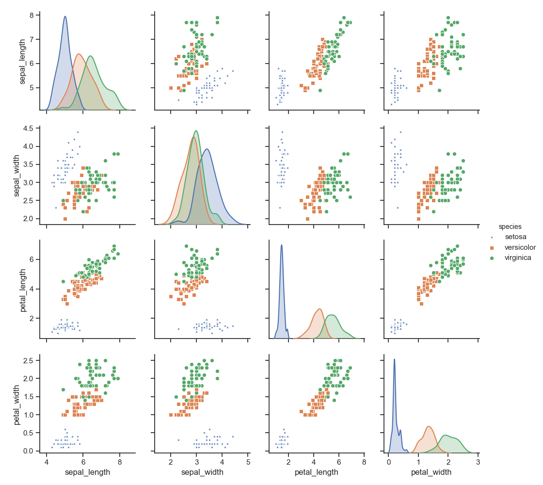
このようになります.一見すると良さげに見えるのですが,解釈するためには勘案しなければならない情報(6つの散布図と4つの正規曲線,つまり対角と上か下三角部分)が多くちょっと手間がかかります.その上De soete and Carroll(1994)では,
including variables that do not contribute much to the clustering structure in the data might obscure the clustering structure or mask it altogether(e.g.,Milligan(1980))
各変数の情報を保ったまま低次元空間でクラスタリングを行うことが理想です.図に表すと,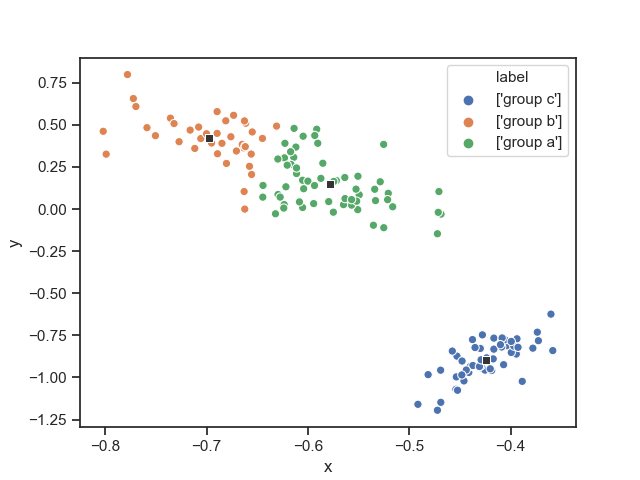
こんな感じ(Reduced K-meansで変数を合成し2次元空間内でクラスタリングした散布図).これができると,
a low-dimensional(say two- or three- dimensional )representations of the cluster structure in X is very useful. Such a representation can aid the researcher in evaluating and interpreting the result of the cluster analysis. For instance, it would allow the researcher to visually inspect the shape of the clusters, to identify outliers, and to assess the degree to which each variable contributes to the cluster structure in the data. (quoted from De soete and Carroll(1994))
といった利点があります(太字の部分が利点です).
これを達成するためにするために,あらかじめ主成分分析で元のデータ行列の変数を合成して,より少数の主成分を構成し,それをクラスタリングするという方法が思い浮かびます.このような,主成分分析$\rightarrow$クラスタリングという分析法を"tandem clustering"(tandem: (英)二段階の)と呼びます.一般的にtandem clusteringはあまり良くないものとされています.
2-2. tandem clustering
じゃあ__tandem clusteringのどこが良くないの?__といった疑問が生まれてきます.De soete and Carroll(1994)では
~ "tandem clustering" has been warned against by several authors(e.g., Arabie and Hubert (in press), Chang (1983), DeSarbo et al. (1990)), because the first few principal components or factors of X do not necessarily define a subspace that is most informative about the cluster structure in the data.
と書かれています.雑に要約すると,主成分分析で合成した第一主成分などは,必ずしも低次元空間でクラスタリングするのに有用な情報を持っているわけではない.つまり,低次元空間を構成する情報とクラスタリングするためにキーとなる情報は必ずしも一致しないということが書かれています.このtandem clusteringの難点を解決する手法がReduced K-meansクラスタリング(以下RKM)です.RKMは次元縮約$\rightarrow$クラスタリングという2ステップを踏むのではなく,__次元縮約とクラスタリングを同時に行う手法__です.低次元に布置するための負荷行列を求めるステップとクラスタリングをするステップとクラスター中心を計算するステップを反復して行うことで,次元縮約とクラスタリングを同時に行なっています.
3. Reduced K-meansのアルゴリズム等について
各パラメータの更新式の導出や詳細なアルゴリズムについては,ざっくりReduced K-meansクラスタリング解説(数理編)にて解説しています.
より詳しく知りたくなった方は,De Soete and Carroll(1994)もしくはTerada(2014)をみてください.
4. 実装例
あいもかわらず汚いコードです.とりあえず,De soete and Carroll(1994)のアルゴリズムで実装しています.Terada(2014)のアルゴリズムで実装したものありますが,ほとんど同じなので載せていません.欲しい方はお声掛けください.
import numpy as np
import matplotlib.pyplot as plt
import seaborn as sns
import pandas as pd

"""
De Soete & Carroll(1994). K-means clustering in a low dimensional Euclidian space

input: data, ndim, ncluster, nstar
data: data matrix for analysis
ndim: ndim means number of dimensions
ncluster: ncluster means number of cluster/centroid
nstar: nstar means number of iteration of choice initial centroid

output: fit, C_hat, E_hat, A, B, X_projected
fit: goodness of fit
C_hat: estimated centroid
E_hat: estimated membership matrix
A: low rank centroid
B: loadings
X_projected: data matrix that projected on low dimensional space
loss_values: a list which contains loss values
"""

# iris dataの散布図行列作成
sns.set(style="ticks")
df = sns.load_dataset("iris")

sns.pairplot(df, hue='species', markers=["*", "s", "o"])
# plt.savefig("/適当なディレクトリ")
plt.show()

def reduced_km(data,ndim,ncluster,nstar=10):
	X = data.astype("float64"); n,p = X.shape
	count = 0;E_hat = np.zeros((n,ncluster));C_hat = np.zeros((ncluster,p))
	loss_best = np.Inf;loss_values = []

	while count < nstar:
		count += 1; print("---------nstart: ",count,"-------------")
		loss = np.Inf
		#initialize cluster mean
		idx = np.random.choice(np.arange(n),ncluster,replace=False)#randomly sample the number of index of object as an initial centroid
		Y = X[idx,]# ncluster * p matrix,
		C = np.copy(Y)# ncluster * p matrix, centroid matrix
		E_old = np.zeros((n,ncluster))
		inner_count = 0
		losses = []
		while True:
			print("%s %d %s %f " % ("inner count ",inner_count,": ",loss))
			inner_count += 1
			# E-step: assign objects to corresponding cluster
			E = np.zeros((n,ncluster))
			for obj in range(n):
				dist_list = []
				for k in range(ncluster):
					dist_list.append(np.sum((X[obj,]-C[k,])**2))
					#print("dist_list[0,",k,"]",dist_list[0,k])
				mindex = np.where(dist_list==np.min(dist_list))#mindex is abbreviation of min_index
				E[obj,mindex] = 1
			W = np.dot(E.T,E);ns = np.diag(W)
			Y = (np.dot(X.T,E)/ns).T

			# C-step:
			WsqrtY = np.dot(np.diag(np.sqrt(ns)),Y)
			U,S,V = np.linalg.svd(WsqrtY, full_matrices=False)
			C = np.dot(np.diag(np.sqrt(1/ns)),np.dot(U[:,:ndim],np.dot(np.diag(S[:ndim]),V[:ndim,:])))

			#evaluation of loss function
			loss_new = np.trace(np.dot((X-np.dot(E,C)).T,(X-np.dot(E,C))))
			losses.append(loss_new)
			diff = loss - loss_new
			if diff < 10**(-8):
				break
			loss = loss_new;
		if loss_new < loss_best:
			loss_best = loss_new
			loss_values = losses
			C_hat = C; E_hat = E
	U,S,V = np.linalg.svd(C_hat,full_matrices=False)
	A = U[:,:ndim];B = np.dot(np.diag(S[:ndim]),V[:ndim,:]).T
	X_projected = np.dot(X,np.dot(V[:ndim,:].T,np.diag(1/S[:ndim])))
	fit = 1 - loss_best/np.trace(np.dot(X.T,X))
	return fit, C_hat, E_hat, A, B, X_projected,loss_values

if __name__ == "__main__":
	from sklearn import datasets
	iris = datasets.load_iris()

	fit, C_hat, E_hat, A, B, X_projected, loss =reduced_km(iris.data,ndim=2,ncluster=3)
	print("%s %f%s" % ("goodness of fit:",100*fit,"%"))
	print("X_projected: \n",X_projected)
	print("low rank Centroid: \n",A)
	loss_df = pd.DataFrame({"loss":loss,"step":list(np.arange(len(loss)))})
	sns.pointplot(x="step",y="loss",data=loss_df,color=".2")
	plt.title("monotonically decreasing loss value")
	plt.show()
	while True:
		if X_projected.shape[1] >= 3:
			print("%s" % ("the dimension is too high to visualize! GOMENNNE!"))
			break
		ans = input("Do you want to visualize projected X? y/n: ")
		if ans == "y":
			lab_name = np.array(["group a","group b","group c"])
			labels = []
			for i in range(X_projected.shape[0]):
				clus_idx = np.where(E_hat[i,]==1)
				labels.append(str(lab_name[clus_idx]))
			labels = pd.DataFrame({"label":labels})
			df_X = pd.DataFrame(X_projected)
			df_X = df_X.rename(columns={0:"x",1:"y"})
			X = pd.concat([df_X,labels],axis=1)
			centroid_df = pd.DataFrame(A);centroid_df = centroid_df.rename(columns={0:"x",1:"y"})
			sns.scatterplot(x="x",y="y",data=X,hue="label",markers=["*","o","+"],legend="full")
			sns.scatterplot(x="x",y="y",data=centroid_df,color=".2",marker="s")
			#plt.savefig("適当なディレクトリ")
			plt.show()
			break
		elif ans == "n":
			break
		else:
			continue
		"""
		注意:

		以上の描画操作はirisデータに対して構成された処理.一般化されていない.

		"""
これをターミナル等で実行すると,先ほどの散布図行列,RKMのプロットに加え,目的関数が単調減少している様子の棒グラフなどが表示されます.変なオプションがついてますが気にしないでください.