10分で学ぶAPPELPY - Pythonの応用計量経済学ライブラリ

10分で学ぶAPPELPY

この投稿はこちらのノートブックの和訳です。

import pandas as pd
import numpy as np
import statsmodels.api as sm  # for datasets
import matplotlib.pyplot as plt
%matplotlib inline

import warnings
warnings.filterwarnings('ignore')

Appelpyの機能をご紹介します。

• 探索的データ分析
• モデル推定
• モデル診断

注意: このノートブックは、Appelpy v0.4.2とその依存関係の最新バージョンを使用して実行されました。

モデルデータセットの設定

それでは、計量経済学の中で最も豊富なデータセットの1つを使って、Appelpyの機能を探ってみましょう。The California Test Score Data Set (Caschool)です。

Pandasでデータセットを読み込み、Statsmodelsメソッドでデータを取得します。

# Load data
df = sm.datasets.get_rdataset('Caschool', 'Ecdat').data
# Add together the two test scores (total score)
df['scrtot'] = df['readscr'] + df['mathscr']

df.head()

	distcod	county	district	grspan	enrltot	teachers	calwpct	mealpct	computer	testscr	compstu	expnstu	str	avginc	elpct	readscr	mathscr	scrtot
0	75119	Alameda	Sunol Glen Unified	KK-08	195	10.900000	0.510200	2.040800	67	690.799988	0.343590	6384.911133	17.889910	22.690001	0.000000	691.599976	690.000000	1381.599976
1	61499	Butte	Manzanita Elementary	KK-08	240	11.150000	15.416700	47.916698	101	661.200012	0.420833	5099.380859	21.524664	9.824000	4.583333	660.500000	661.900024	1322.400024
2	61549	Butte	Thermalito Union Elementary	KK-08	1550	82.900002	55.032299	76.322601	169	643.599976	0.109032	5501.954590	18.697226	8.978000	30.000002	636.299988	650.900024	1287.200012
3	61457	Butte	Golden Feather Union Elementary	KK-08	243	14.000000	36.475399	77.049202	85	647.700012	0.349794	7101.831055	17.357143	8.978000	0.000000	651.900024	643.500000	1295.400024
4	61523	Butte	Palermo Union Elementary	KK-08	1335	71.500000	33.108601	78.427002	171	640.849976	0.128090	5235.987793	18.671329	9.080333	13.857677	641.799988	639.900024	1281.700012

データを検査する

データを手に入れたので、モデリングを行う前に、いくつかの主要な変数の分布について詳しく調べてみましょう。

Appelpyには、edaモジュール (探索的データ分析)があります。

from appelpy.eda import statistical_moments

すべての統計的モーメントを一度に取得します。
1. 平均
2. 分散
3. 歪度（デフォルトはフィッシャー）
4. 尖度

statistical_moments(df)

	mean	var	skew	kurtosis
distcod	67472.8	1.20201e+07	-0.0307844	-1.09626
enrltot	2628.79	1.53124e+07	2.87017	10.2004
teachers	129.067	35311.2	2.93254	11.219
calwpct	13.246	131.213	1.68306	4.58959
mealpct	44.7052	735.678	0.183954	-0.999802
computer	303.383	194782	2.87169	10.7729
testscr	654.157	363.03	0.0916151	-0.254288
compstu	0.135927	0.00421926	0.922369	1.43113
expnstu	5312.41	401876	1.0679	1.87571
str	19.6404	3.57895	-0.0253655	0.609597
avginc	15.3166	52.2135	2.21516	6.53212
elpct	15.7682	334.375	1.4268	1.4354
readscr	654.97	404.331	-0.0583962	-0.358049
mathscr	653.343	351.72	0.255082	-0.159811
scrtot	1308.31	1452.12	0.0916149	-0.254288

モデルの推定

Appelpyの中核となるのは、データセットの中の現象をモデル化することです。

linear_model モジュールは、データをモデル化するためのクラスを含んでいます。例：OLS（Ordinary Least Squares）

from appelpy.linear_model import OLS

線形モデルを推定するためのレシピを紹介します。

1. 従属変数(y)と独立変数(X)のために、y_list と X_list の2つのリストを作成します。

y_list = ['scrtot']
X_list = ['avginc', 'str', 'enrltot', 'expnstu']

1. モデルのデータフレームと2つのリストをOLSオブジェクトの入力として渡すことで、1行でモデルをフィットします。

model_nonrobust = OLS(df, y_list, X_list).fit()

1. 二乗平均平方根誤差(Root MSE)を含む、model_selection_stats属性でキーモデルの結果を取得します。

model_nonrobust.model_selection_stats

{'root_mse': 25.85923055850994,
 'r_squared': 0.5438972040191434,
 'r_squared_adj': 0.5395010324916171,
 'aic': 3929.1191674301117,
 'bic': 3949.320440986499}

Statsmodels のサマリーを results_output 属性で取得します...

model_nonrobust.results_output

OLS Regression Results

Dep. Variable:	scrtot	R-squared:	0.544
Model:	OLS	Adj. R-squared:	0.540
Method:	Least Squares	F-statistic:	123.7
Date:	Mon, 04 May 2020	Prob (F-statistic):	2.05e-69
Time:	18:32:26	Log-Likelihood:	-1959.6
No. Observations:	420	AIC:	3929.
Df Residuals:	415	BIC:	3949.
Df Model:	4
Covariance Type:	nonrobust

	coef	std err	t	P>|t|	[0.025	0.975]
const	1312.9203	27.833	47.171	0.000	1258.208	1367.632
avginc	3.8640	0.185	20.876	0.000	3.500	4.228
str	-1.3954	0.893	-1.563	0.119	-3.150	0.359
enrltot	-0.0016	0.000	-4.722	0.000	-0.002	-0.001
expnstu	-0.0061	0.003	-2.316	0.021	-0.011	-0.001

Omnibus:	7.321	Durbin-Watson:	0.763
Prob(Omnibus):	0.026	Jarque-Bera (JB):	7.438
Skew:	-0.326	Prob(JB):	0.0243
Kurtosis:	2.969	Cond. No.	1.39e+05

Warnings:
[1] Standard Errors assume that the covariance matrix of the errors is correctly specified.
[2] The condition number is large, 1.39e+05. This might indicate that there are
strong multicollinearity or other numerical problems.

...これでようやく results_output_standardized 属性を使って標準化されたモデルの結果を簡単に取得できるようになりました。

model_nonrobust.results_output_standardized
# This is a Styler object; add .data to access the underlying Pandas dataframe

Unstandardized and Standardized Estimates

	coef	t	P>|t|	coef_stdX	coef_stdXy	stdev_X
scrtot
avginc	+3.8640	+20.876	0.000	+27.9209	+0.7327	7.2259
str	-1.3954	-1.563	0.119	-2.6399	-0.0693	1.8918
enrltot	-0.0016	-4.722	0.000	-6.3035	-0.1654	3913.1050
expnstu	-0.0061	-2.316	0.021	-3.8364	-0.1007	633.9371

出力はStataのlistcoefコマンドと似ています。

モデルの診断

モデルオブジェクトの diagnostic_plot メソッドを呼び出して、多くの視覚的な 回帰診断を表示します:。

• pp_plot: P-P プロット
• qq_plot: Q-Q プロット
• rvp_plot: 残差と予測値のプロット
• rvf_plot: 残差と実測値のプロット

Appelpyの diagnostics モジュールは、回帰診断のためのクラスと関数のスイートを持っています。

• 視覚的な診断だけでは十分でない場合は、heteroskedasticity_testのような他のメソッドを呼び出して正式なテストを行います。

• モデルを汚している観測値はありますか？ モデルオブジェクトを BadApples クラスに渡して、影響力のある点、外れ値、高レバレッジの点を調べます。

描画

診断プロットの2x2セットのレシピがこちらにあります。

fig, axarr = plt.subplots(2, 2, figsize=(10, 10))
model_nonrobust.diagnostic_plot('pp_plot', ax=axarr[0][0])
model_nonrobust.diagnostic_plot('qq_plot', ax=axarr[1][0])
model_nonrobust.diagnostic_plot('rvf_plot', ax=axarr[1][1])
axarr[0, 1].axis('off')
plt.tight_layout()

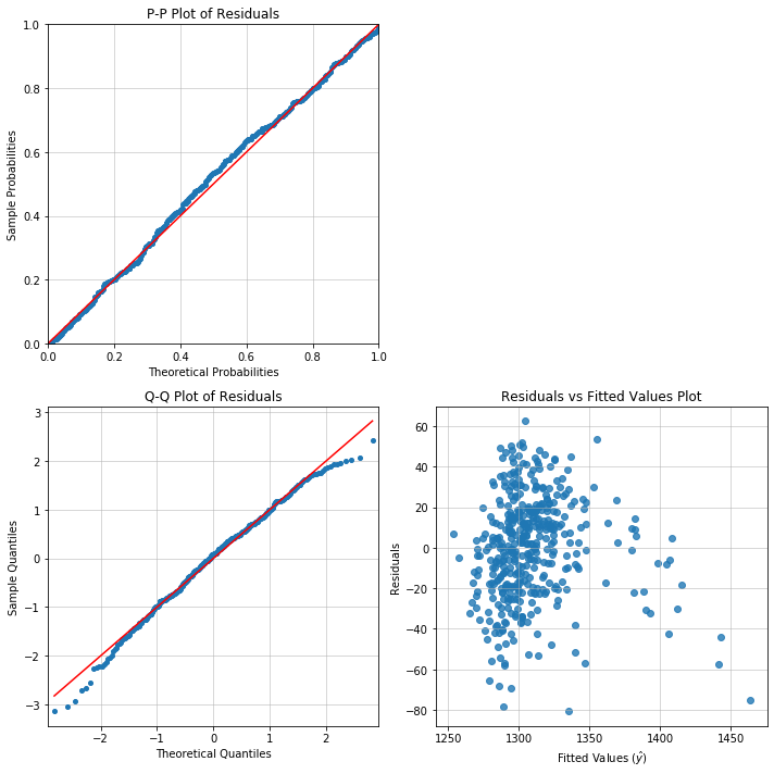
やれやれ。指定されたモデルには1350以上のテストスコアに 特別な問題があります。

RVFプロットに一定でない分散があるようです。

おそらく等分散性もあると思いますが、もっと具体的なテストをしてみましょう。

等分散性

from appelpy.diagnostics import heteroskedasticity_test

いくつかの 等分散性検定 のいずれかを呼び出します。例：
- Breusch-Pagan (Stataの hettest コマンドのデフォルト)
- Bresuch-Pagan studentized (Rの bptest コマンドのデフォルト)
- White (Stataの hettest, white コマンド)

bp_stats = heteroskedasticity_test('breusch_pagan', model_nonrobust)
print('Breusch-Pagan test :: {}'.format(bp_stats['distribution'] + '({})'.format(bp_stats['nu'])))
print('Test statistic: {:.4f}'.format(bp_stats['test_stat']))
print('Test p-value: {:.4f}'.format(bp_stats['p_value']))

Breusch-Pagan test :: chi2(1)
Test statistic: 2.5579
Test p-value: 0.1097

bps_stats = heteroskedasticity_test('breusch_pagan_studentized', model_nonrobust)
print('Breusch-Pagan test (studentized) :: {}'.format(bps_stats['distribution'] + '({})'.format(bps_stats['nu'])))
print('Test statistic: {:.4f}'.format(bps_stats['test_stat']))
print('Test p-value: {:.4f}'.format(bps_stats['p_value']))

Breusch-Pagan test (studentized) :: chi2(1)
Test statistic: 11.3877
Test p-value: 0.0225

Studentized Breusch-Pagan検定は、よりロバストであると見なされ、等分散性の初期仮説との有意差を示しているので、Heteroskedastic-Robust標準誤差（ HC1誤差）をもつモデルに適合させましょう。

model_hc1 = OLS(df, y_list, X_list, cov_type='HC1').fit()

model_hc1.results_output

OLS Regression Results

Dep. Variable:	scrtot	R-squared:	0.544
Model:	OLS	Adj. R-squared:	0.540
Method:	Least Squares	F-statistic:	78.60
Date:	Mon, 04 May 2020	Prob (F-statistic):	1.36e-49
Time:	18:32:27	Log-Likelihood:	-1959.6
No. Observations:	420	AIC:	3929.
Df Residuals:	415	BIC:	3949.
Df Model:	4
Covariance Type:	HC1

	coef	std err	z	P>|z|	[0.025	0.975]
const	1312.9203	29.364	44.711	0.000	1255.367	1370.474
avginc	3.8640	0.240	16.119	0.000	3.394	4.334
str	-1.3954	0.932	-1.498	0.134	-3.221	0.430
enrltot	-0.0016	0.000	-5.794	0.000	-0.002	-0.001
expnstu	-0.0061	0.003	-2.166	0.030	-0.012	-0.001

Omnibus:	7.321	Durbin-Watson:	0.763
Prob(Omnibus):	0.026	Jarque-Bera (JB):	7.438
Skew:	-0.326	Prob(JB):	0.0243
Kurtosis:	2.969	Cond. No.	1.39e+05

Warnings:
[1] Standard Errors are heteroscedasticity robust (HC1)
[2] The condition number is large, 1.39e+05. This might indicate that there are
strong multicollinearity or other numerical problems.

今、有意な回帰子（独立変数）は何でしょうか？

model_hc1.significant_regressors(0.05)

['avginc', 'enrltot', 'expnstu']

str (student-teacher ratio) と expnstu の回帰子は、特に生徒への投資に関連しています。 2つの回帰子が一緒になって0から有意に異なるかどうかを検定するために、Wald検定 を行うことができます。

from appelpy.diagnostics import wald_test

wald_stats = wald_test(model_hc1, ['str', 'expnstu'])
print('Wald test :: {}'.format(wald_stats['distribution'] + '({})'.format(wald_stats['nu'])))
print('Test statistic: {:.4f}'.format(wald_stats['test_stat']))
print('Test p-value: {:.4f}'.format(wald_stats['p_value']))

Wald test :: chi2(2)
Test statistic: 4.7352
Test p-value: 0.0937

一部の変数の標準誤差が、非ロバスト誤差と比較して、HC1誤差の方が高いのは当然のことです。

pd.concat([pd.Series(model_nonrobust.results.bse, name='std_error_nonrobust'),
           pd.Series(model_hc1.results.bse, name='std_error_hc1')], axis='columns')

	std_error_nonrobust	std_error_hc1
const	27.833430	29.364467
avginc	0.185093	0.239715
str	0.892703	0.931541
enrltot	0.000341	0.000278
expnstu	0.002613	0.002794

異常な観測値：レバレッジ、外れ値、そして影響力

観察した結果を検査してみましょう。

• 高い影響力
• 高いレバレッジ
• 外れ値

from appelpy.diagnostics import BadApples

モデルオブジェクトを用いて BadApples のインスタンスを設定する。

bad_apples = BadApples(model_hc1).fit()

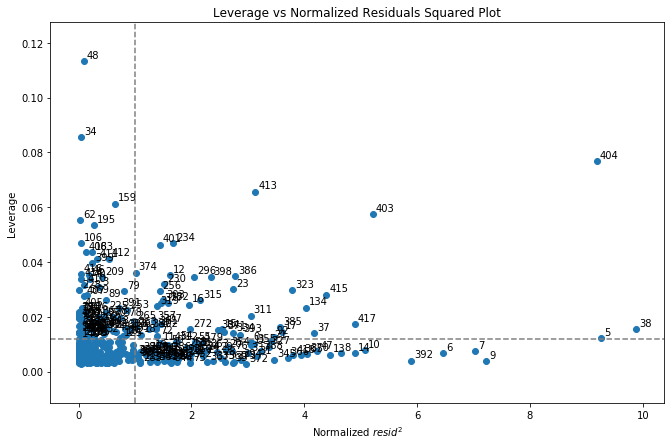
正規化された残差の2乗に対してレバレッジ値をプロットしてみましょう。

右上の象限にある観測値は、平均よりも高いレバレッジ値と残差値を持っています（つまり、モデルで最も影響力のある観測値です）。

fig, ax = plt.subplots(figsize=(11,7))
bad_apples.plot_leverage_vs_residuals_squared(annotate=True)
plt.show()

レバレッジ

レバレッジの値は measures_leverage 属性に格納されます。

bad_apples.measures_leverage.sort_values(ascending=False).head()

48     0.113247
34     0.085633
404    0.076762
413    0.065741
159    0.061353
Name: leverage, dtype: float64

レバレッジが最も高い5つの観測値を見てみましょう。

bad_apples.show_extreme_observations().loc[[48,34,404,413,159]]

	scrtot	avginc	str	enrltot	expnstu
48	1261.099976	12.109128	19.017494	27176	5864.366211
34	1252.200012	11.722225	21.194069	25151	5117.039551
404	1387.900024	55.327999	16.262285	1059	6460.657227
413	1398.200012	50.676998	15.407042	687	7217.263184
159	1294.500000	14.298300	20.291372	21338	5123.474121

model_hc1.X_standardized.loc[[48,34,404,413,159]]

	avginc	str	enrltot	expnstu
48	-0.443884	-0.329278	6.273077	0.870684
34	-0.497428	0.821246	5.755585	-0.308182
404	5.537230	-1.785664	-0.401163	1.811299
413	4.893572	-2.237740	-0.496228	3.004803
159	-0.140922	0.344087	4.781167	-0.298032

これらの高レバレッジな点は、少なくとも1つの独立変数が平均値から4標準偏差以上離れた値を持っています。

外れ値

BadApplesオブジェクトは、尺度の値が「極端」であるかどうかを判断するためのヒューリスティックを計算します。

極端なインデックスは属性に格納され、例えば外れ値は indices_outliers に格納されます。

bad_apples.indices_outliers

[5, 6, 7, 8, 9, 10, 13, 14, 37, 38, 47, 134, 370, 392, 403, 404, 415, 417]

外れ値のヒューリスティック：標準化された残差の絶対値またはスチューデント化された残差の絶対値が2より大きい場合、観測値は外れ値です。

print(f"Proportion of observations as outliers: {len(bad_apples.indices_outliers) / len(df):.4%}")

Proportion of observations as outliers: 4.2857%

そのヒューリスティックにより、観測値の約5％以下が外れ値と見なされると予想されます。

影響力

また、クックの距離、dffits、dfbetaなどの様々な影響力測定も考慮してください。

bad_apples.measures_influence.sort_values('cooks_d', ascending=False).head()

	dfbeta_const	dfbeta_avginc	dfbeta_str	dfbeta_enrltot	dfbeta_expnstu	cooks_d	dffits_internal	dffits
404	0.010742	-0.811324	0.068295	0.061925	0.039761	0.152768	-0.873981	-0.882753
403	0.024082	-0.529623	0.016131	0.031978	0.026944	0.063718	-0.564440	-0.567338
413	0.074297	-0.373064	0.013021	0.033955	-0.099557	0.044116	-0.469661	-0.470876
38	-0.277356	-0.193382	0.217223	-0.136237	0.315817	0.030955	-0.393412	-0.397701
415	-0.157629	0.099707	0.045684	-0.026836	0.249169	0.025414	0.356468	0.357936

要約

• データセットをロードし、Pandasで前処理を行います。
• Appelpy eda: 統計モーメントなどの便利な関数でモデルデータセットを検査します。
• Appelpy modelling. linear_modelには、モデル推定のためのOLSやWLSなどのクラスが含まれています。 各モデルの短いレシピを使用して、モデルの推定値にアクセスします。
• Appelpy diagnostics: モデル推定値が有効かどうかを、診断プロット、統計的検定、影響力分析のためのBadApplesなどの診断でチェックします。

その他の機能もチェックしてみましょう。

• ロジスティック回帰 (discrete_model の下)
• DummyEncoder と InteractionEncoder クラス