Introduction to Econometrics with Rの練習問題をPythonで解いてみます。
2.3 練習問題 - 確率論
1. サンプリング
宝くじで$ 49 $のうち$ 6 $ つのユニークな数字が抽選されます。
指示:
今週の当選番号を引きなさい。
import math

import numpy as np
import matplotlib.pyplot as plt
%matplotlib inline

from scipy import integrate, stats
np.random.seed(seed=123)
np.random.randint(low=1, high=50, size=6)
array([46, 3, 29, 35, 39, 18])
2. 確率密度関数
以下の確率密度関数 (PDF)を用いて、ランダムな変数 $X$ を考えなさい。
$$f_X(x)=\frac{x}{4}e^{-x^2/8},\quad x\geq 0.$$
指示:
上記の確率密度関数を関数 f()として定義せよ。
定義した関数が、実際に確率密度関数であることを確認せよ。
def f(x):
    return x/4*math.exp(-x**2/8)

integrate.quad(f, 0, np.inf)
(1.0, 2.1730298600934144e-09)
3. 期待値と分散
この練習問題では、前の練習問題で考えたランダムな変数 $X$ の期待値と分散を計算しなければなりません。
前の練習問題の確率密度関数 f() は動作環境で利用可能なものとします。
指示:
積分すると $X$ の期待値になる適切な関数 ex() を定義せよ。
$X$ の期待値を計算せよ。結果を expected_value に格納せよ。
積分すると $X^2$ の期待値になる適切な関数 ex2() を定義せよ。
$X$ の分散を計算せよ。結果を variance に格納せよ。
# define the function ex
def ex(x):
    return x*f(x)

# compute the expected value of X
expected_value = integrate.quad(ex, 0, np.inf)[0]

# define the function ex2
def ex2(x):
    return x**2*f(x)

# compute the variance of X
variance = integrate.quad(ex2, 0, np.inf)[0] - expected_value**2
4. 標準正規分布 I
Let $Z\sim\mathcal{N}(0, 1)$.
指示:
$\phi(3)$, つまり、$c=3$ での標準正規密度の値を計算せよ。
stats.norm.pdf(3)
0.0044318484119380075
5. 標準正規分布 II
Let $Z\sim\mathcal{N}(0, 1)$.
指示:
$P(|Z|\leq 1.64)$ を計算せよ。
# compute the probability
stats.norm.cdf(1.64) - stats.norm.cdf(-1.64)
0.8989948330517925
6. 正規分布 I
Let $Y\sim\mathcal{N}(5, 25)$.
指示:
与えられた分布の99%分位を計算せよ、すなわち、$y$ が $\Phi(\frac{y-5}{5})=0.99$ となるような $y$ を見つけよ。
# compute the 99% quantile of a normal distribution with mu = 5 and sigma^2 = 25.
stats.norm.ppf(0.99, 5, np.sqrt(25))
16.631739370204205
7. 正規分布 II
Let $Y\sim\mathcal{N}(2, 12)$.
指示:
この分布から$10$の乱数を生成せよ。
# generate 10 random numbers from the given distribution.
stats.norm.rvs(loc=2, scale=np.sqrt(12), size=10, random_state=12)
array([ 3.63847098, -0.36052849,  2.83983505, -3.89152106,  4.60896331,
       -3.31643067,  2.01776072,  1.58351913, -0.79546723, 11.9482742 ])
8. カイ二乗分布 I
Let $W\sim\chi^2_{10}$.
指示:
対応する確率密度関数をプロットせよ。x値の範囲を$[0,25]$に指定せよ。
# plot the PDF of a chi^2 random variable with df = 10

x = np.arange(0, 25)
plt.plot(x, stats.chi2.pdf(x, df=10))
plt.show()

9. カイ二乗分布 II
Let $X_1$ and $X_2$ be two independent normally distributed random variables with $\mu=0$ and $\sigma^2=15$.
指示:
$P(X_1^2+X_2^2>10)$ を計算せよ。
# compute the probability

stats.chi2.sf(10/15, df=2, loc=0, scale=1)
0.7165313105737892
10. スチューデントのt分布 I
Let $X\sim t_{10000}$ and $Z\sim\mathcal{N}(0,1)$.
指示:
両方の分布の $95%$分位を計算せよ。何か発見があるか?
# compute the 95% quantile of a t distribution with 10000 degrees of freedom
# qt(0.95, df = 10000)

print(stats.t.ppf(0.95, df = 10000))

# compute the 95% quantile of a standard normal distribution

print(stats.norm.ppf(0.95))

# both values are very close to each other. This is not surprising as for sufficient large degrees of freedom the t distribution can be approximated by the standard normal distribution.
1.6450060180692423
1.6448536269514722
11. スチューデントのt分布 II
Let $X\sim t_1$. Once the session has initialized you will see the plot of the corresponding probability density function (PDF).
指示:
この分布から$1000$の乱数を生成し、変数xに代入せよ。
xの標本平均を計算せよ。結果を説明でるか?
# generate 1000 random numbers from the given distribution. Assign them to the variable x.
x = stats.t.rvs(df = 1, size = 1000, random_state = 1)

# compute the sample mean of x.
np.mean(x)

# Although a t distribution with M = 1 is, as every other t distribution, symmetric around zero it actually has no expectation. This explains the highly non-zero value for the sample mean.
10.845661965991818
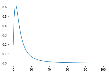
12. F分布 I
Let $Y\sim F(10, 4)$.
指示:
与えられた分布の分位関数をプロットせよ。
# plot the quantile function of the given distribution

dfn = 10
dfd = 4

x = np.linspace(stats.f.ppf(0.01, dfn, dfd),
                stats.f.ppf(0.99, dfn, dfd), 100)

plt.plot(stats.f.pdf(x = x, dfn = dfn, dfd = dfd))
plt.show()
13. F分布 II
Let $Y\sim F(4,5)$.
指示:
確率密度関数を積分して $P(1<Y<10)$ を計算せよ。
# compute the probability by integration

dfn = 4
dfd = 5

x = np.linspace(stats.f.ppf(0.01, dfn, dfd),
                stats.f.ppf(0.99, dfn, dfd), 100)

def function(x):
    return stats.f.pdf(x = x, dfn = dfn, dfd = dfd)

integrate.quad(function, 1, 10)[0]
0.4723970230052129