This is a memorandum to remind myself how the code of arbitrary gaussian distribution generation works.
To generate multiple gaussian distributions, it's a good idea to employ trigonometric functions.
from math import cos, sin
import numpy as np
import matplotlib.pyplot as plt

# prepare variables
label = 1 # index of an individual distribution
n_labels = 6 # total number of distributions
x = np.random.normal(0, 1, (1000,1)) # x coord. of random numbers
y = np.random.normal(0, 1, (1000,1)) # y coord. of random numbers

# define the angle for each distribution
r = 2.0 * np.pi / float(n_labels) * float(label)
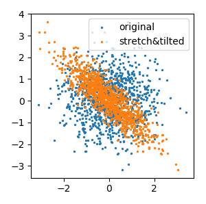
To stretch and tile the distribution, you can do this:
new_x = x * cos(r) - y * sin(r)
plt.figure(figsize=(3, 3))
plt.scatter(x, y, s=2)
plt.scatter(new_x, y, s=2)
plt.legend(['original', 'stretch&tilted'])
plt.show()
then, you'll get following result:
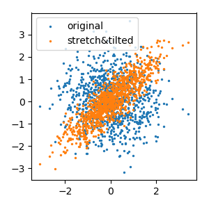
You can do the same to y coordinate as well.
new_y = x * sin(r) + y * cos(r)
plt.figure(figsize=(3, 3))
plt.scatter(x, y, s=2)
plt.scatter(x, new_y, s=2)
plt.legend(['original', 'stretch&tilted'])
plt.show()
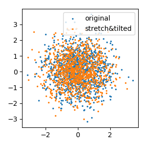
If you use both new_x and new_y, the distribution will be a normal one.
plt.figure(figsize=(3, 3))
plt.scatter(x, y, s=2)
plt.scatter(new_x, new_y, s=2)
plt.legend(['original', 'stretch&tilted'])
plt.show()
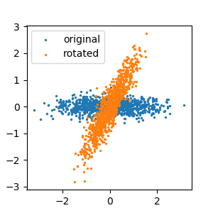
This is useful when the standard deviations of the distribution in x and y coordinates are different.
x1 = np.random.normal(0, 1, (1000,1))
y1 = np.random.normal(0, 0.2, (1000,1))
new_x1 = x1 * cos(r) - y1 * sin(r)
new_y1 = x1 * sin(r) + y1 * cos(r)

plt.figure(figsize=(3, 3))
plt.scatter(x1, y1, s=2)
plt.scatter(new_x1, new_y1, s=2)
plt.legend(['original', 'rotated'])
plt.show()
You can add some shift to the whole distribution towards a certain direction defined by r that we have defined previously.
shift = 2 # the amount of shift
new_x += shift * cos(r) # parallel shift to the direction of r
new_y += shift * sin(r) # parallel shift to the direction of r
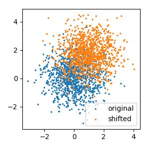
You can make it as a function for convenience.
def sample(x, y, label, n_labels, shift):
    r = 2.0 * np.pi / float(n_labels) * float(label)
    new_x = x * cos(r) - y * sin(r) # change the slope of the distribution
    new_y = x * sin(r) + y * cos(r) # change the slope of the distribution
    new_x += shift * cos(r) # parallel shift to the direction of r
    new_y += shift * sin(r) # parallel shift to the direction of r
    return np.concatenate((new_x, new_y), axis=1)

new_xy = sample(x,y,1,6,2)

plt.figure(figsize=(3,3))
plt.scatter(x,y,s=2)
plt.scatter(new_xy[:,0],new_xy[:,1],s=2)
plt.legend(['original','shifted'])
plt.show()
plt.tight_layout()
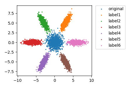
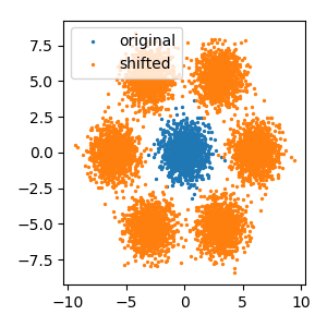
Let's make a circle of 6 gaussian distributions!
n_labels = 6
new_xy = np.empty((0,2))
for i in range(n_labels):
    a = sample(x, y, i+1, n_labels, 6)
    new_xy = np.concatenate((new_xy, a), axis=0)
We can also give each distribution a different label
n_labels = 6
plt.figure(figsize=(4.5, 3))
plt.scatter(x, y, s=2, label='original')
for i in range(n_labels):
    x1 = np.random.normal(0, 1, (1000,1))
    y1 = np.random.normal(0, 0.3, (1000,1))
    new_xy = sample(x1, y1, i+1, n_labels, 6)
    plt.scatter(new_xy[:,0], new_xy[:,1],
                s=2, label='label{}'.format(i+1))
plt.legend(bbox_to_anchor=(1.05, 1),
           loc='upper left', borderaxespad=0)
plt.show()
plt.tight_layout()