Pythonを使って東京都家賃についての研究 (3の2)

結果抜粋

ブログに同時掲載：
https://leoluistudio.com/blog/24/python%e3%82%92%e4%bd%bf%e3%81%a3%e3%81%a6%e6%9d%b1%e4%ba%ac%e9%83%bd%e5%ae%b6%e8%b3%83%e3%81%ab%e3%81%a4%e3%81%84%e3%81%a6%e3%81%ae%e7%a0%94%e7%a9%b6-4%e3%81%ae2/

統計の手法1

データ収集

• データ元：https://suumo.jp
• 使ったライブラリ：requests, BeautifulSoup, re, time, sqlite3
• 収集の部分がただrequestしてデータベースに入れるだけなのでコードを割愛します

---

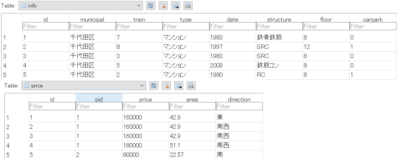
データベース

データベースの構造

info
id	1 (PRIMARY KEY)
municipal	千代田区
train	7 (駅まで徒歩)
type	マンション
date	1983
structure	鉄骨鉄筋
floor	8
carpark	0 (0は無・1は有)

price
id	1 (PRIMARY KEY)
pid	160000 (円)
1 (= infoのid)	7 (駅まで徒歩)
area	42.9 (平米)
date	東

テーブル毎に最初の5行目

---

プログラムと結果

まず必要なライブラリーを導入

import sqlite3
import pandas as pd

import plotly.express as px
import plotly.graph_objects as go
from plotly.offline import plot

from sklearn.decomposition import PCA

---

データベースを接続する

# 結果を出力だけの場合
conn = sqlite3.connect(‘info.db’)
c = conn.cursor()
cursor = c.execute(“SQLコード”)
for row in cursor:
    print(結果)
conn.close()

# 結果を保存して処理の場合
conn = sqlite3.connect(‘info.db’)
df = pd.read_sql_query(“SQLコード”, conn)
conn.close()

---

最初はデータの分布を見る

# infoの行数
SELECT COUNT(id) FROM info
# 結果：82,812

# priceの行数
SELECT COUNT(id) FROM price
# 結果：624,499

# 「アパート」と「マンション」の数
SELECT type,COUNT(type) FROM info GROUP BY type
# 結果：アパート 33,110 / マンション 49,702

---

完成日の分布

# SQL
SELECT date AS year,COUNT(date) AS count FROM info WHERE date > 0 GROUP BY date

# グラフ
fig = px.bar(df, x=’year’, y=’count’, height=500, width=1000)

---

建物構造の分布

# SQL
SELECT structure,COUNT(structure) AS count FROM info WHERE structure != 0 GROUP BY structure

# グラフ
fig = px.bar(df, x=structure, y=’count’, height=500, width=1000)

---

階数の分布

# SQL
SELECT floor,COUNT(floor) AS count FROM info WHERE floor != 0 GROUP BY floor

# グラフ
fig = px.bar(df, x=floor, y=’count’, height=500, width=1000)

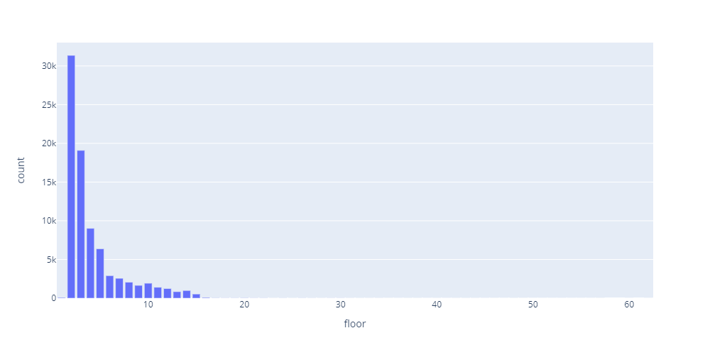
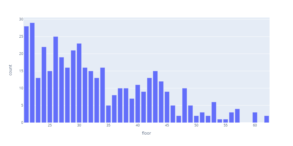
上の表で20階以上の分布が全く見えないのでこちらで細かく見ていきます。

# SQL
SELECT floor,COUNT(floor) AS count FROM info WHERE floor > 20 GROUP BY floor

# グラフ
fig = px.bar(df, x=floor, y=’count’, height=500, width=1000)

---

連続型変数 (e.g. 価格) を分析する前にグループに分ける必要があります。

def pricegroup(df):
    if df[‘price’] < 30000:
      return ‘<30,000’
    elif df[‘price’] < 60000:
      return ‘30,000-60,000’
    ……
    else:
      return ‘>270,000’

pricegroup_list = [‘<30,000’,
    ‘30,000-60,000’,
    ‘60,000-90,000’,
    ……
    ‘240,000-270,000’,
    ‘>270,000’]

価格の分布

# SQL
SELECT price FROM price

# Dataframeの処理df[‘pricegroup’] = df.apply(pricegroup, axis=1)
dfcount = df.groupby([‘pricegroup’]).count()

#グラフ
fig = px.bar(dfcount, x=dfcount.index, y=’price’, height=500, width=1000)
fig.update_layout(xaxis={‘categoryorder’:’array’, ‘categoryarray’:pricegroup_list}, yaxis_title=’count’)

---

面積の分布も同じくように

def pricegroup(df):
    if df[‘area’] < 5:
      return ‘<5’
    elif df[‘area’] < 10:
      return ‘5-10’
    ……
    else:
      return ‘>45’

pricegroup_list = [‘<5′, ’5-10′, ’10-15′, ’15-20′,
    ’20-25′, ’25-30′, ’30-35′, ’35-40′,
    ’40-45′,’>45′]

# SQL
SELECT area FROM price

# Dataframeの処理
df[‘areagroup’] = df.apply(areagroup, axis=1)
dfcount = df.groupby([‘areagroup’]).count()

# グラフ
fig = px.bar(dfcount, x=dfcount.index, y=’area’, height=500, width=1000)
fig.update_layout(xaxis={‘categoryorder’:’array’, ‘categoryarray’:areagroup_list}, yaxis_title=’count’)

---

方向の分布

# SQL
SELECT direction,COUNT(direction) AS count FROM price WHERE direction != ‘-‘ GROUP BY direction

# グラフ
fig = px.bar(df, x=direction, y=’count’, height=500, width=1000)

---

区市町村の分析をする前に23区と市部に分けます。

m23_list = [‘千代田区’,’中央区’,’港区’,’新宿区’,’文京区’,’台東区’,’墨田区’,
    ‘江東区’,’品川区’,’目黒区’,’大田区’,’世田谷区’,’渋谷区’,’中野区’,
    ‘杉並区’,’豊島区’,’北区’,’荒川区’,’板橋区’,’練馬区’,’足立区’,
    ‘葛飾区’,’江戸川区’]

municipal_dict = {}
conn = sqlite3.connect(‘info.db’)
c = conn.cursor()
cursor = c.execute(“SELECT id,municipal FROM info”)
for row in cursor:
    municipal_dict.update({row[0]:row[1]})
conn.close()

def municipal(df):
    return municipal_dict[df[‘pid’]]

def municipal23(df):
    if df[‘municipal’] in m23_list:
      return ‘Special Wards’
    else:
      return ‘Non Special Wards’

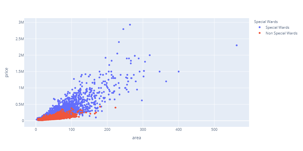
価格と面積の関係（23区と市部に分ける）

# SQL
SELECT pid,price,area FROM price

# Dataframeの処理
df[‘municipal’] = df.apply(municipal, axis=1)
df[‘municipal23’] = df.apply(municipal23, axis=1)
dfmedian = df.groupby([‘pid’, ‘municipal23’])[‘price’, ‘area’].median()
dfmedian_reset = dfmedian.reset_index(level=’municipal23′)

# グラフ
fig = px.scatter(dfmedian_reset, x=’area’, y=’price’, color=’municipal23′, labels={‘municipal23’: ‘Special Wards’}, height=500, width=1000)