深層学習とChemoinformatics
近年, ケモインフォマティクス分野では化学構造に対する深層学習が話題です. 本記事では, PyTorch geometricを用いたGraph Convolutional Networks (GCN) による溶解度予測を実装します. 分子中の原子プロパティやその隣接原子との結合関係から分子の物性・薬理活性・毒性などを予測することが可能であり, 創薬への応用などが期待できます.
1. Graph Convolutional Network
1.1 Graph
グラフ$\mathcal{G}$は, 頂点とそれらの結びつき(エッジ)で表される$\mathcal{G=(V, E)}$のことを指します.
ここで,$\mathcal{V}=\{v_{1}, v_{2}, \ldots, v_{i}\}$は頂点$v$の集合, $\mathcal{E}=\{e_{11}, e_{12}, \ldots, e_{ij}\}$はエッジ$e$の集合です. 頂点同士の結びつきに方向性がない場合を無向グラフ(左図), 方向性がある場合を有向グラフ(右図)と呼びます.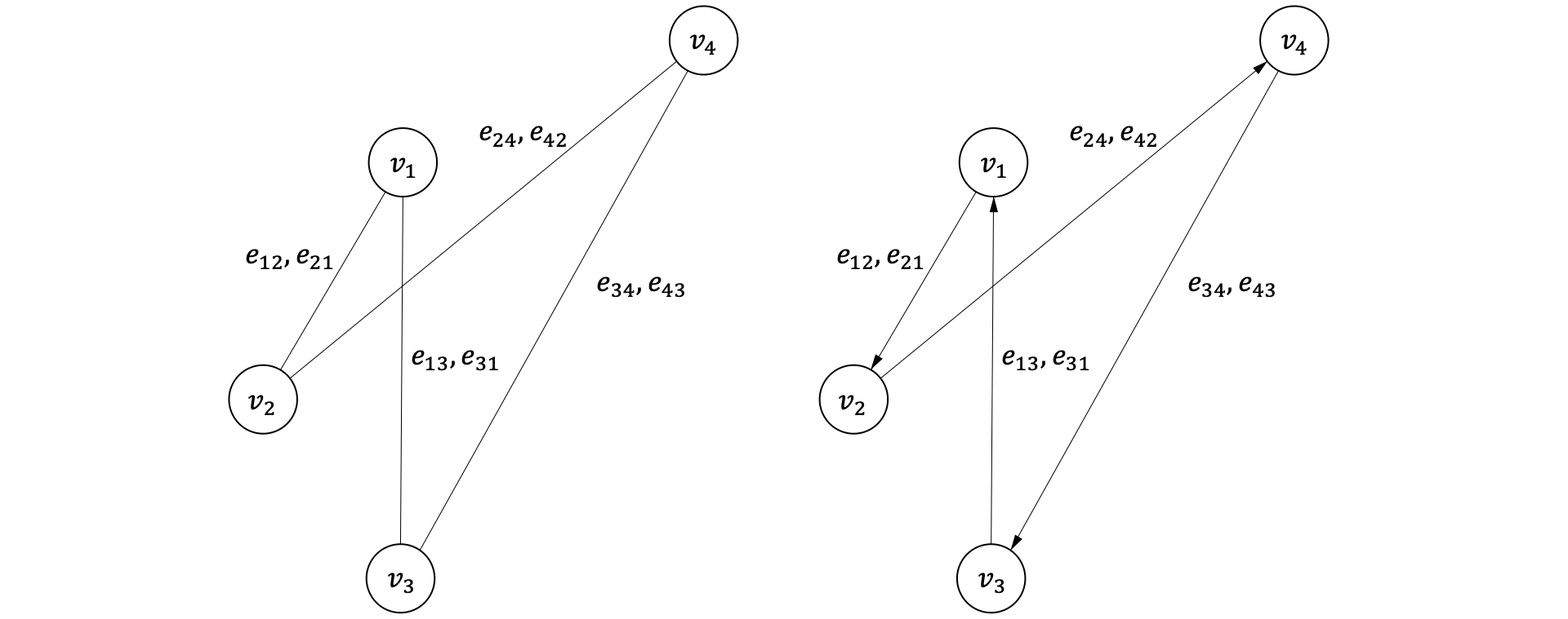
化合物は原子を頂点とし, それらがエッジによって結びつけられた無向グラフと見なすことが可能です. そのためこの記事では無向グラフのみ取り扱います.
1.2 隣接行列と特徴行列
頂点数$n$の無向グラフ$\mathcal{G}$が与えられた時, $\mathcal{G}$の頂点の結合関係は, 隣接行列 $\boldsymbol{A}\in \mathbb{R}^{n\times n}$で表すことが可能です. 上図の例だと, $\boldsymbol{A}$は以下のようになります.
\begin{eqnarray}
A = \left(
\begin{array}{cccc}
0 & 1 & 1 & 0\\
1 & 0 & 0 & 1\\
1 & 0 & 0 & 1\\
0 & 1 & 1 & 0
\end{array}
\right)
\end{eqnarray}
A_{ij} = \left\{
\begin{array}{ll}
1 & \rm{if\,ij\,bond} \\
0 & \rm{else\,}
\end{array}
\right.
$$ここで, $\boldsymbol{A}$の行および列は各頂点の番号に対応しております. $\boldsymbol{A}$の中身は頂点同士が結合している場合1, 結合していない場合は0の値を持ちます.
また各頂点が特徴量として$k$次元のベクトルを有するとき, $\mathcal{G}$の各頂点の特徴量は特徴行列$\boldsymbol{X}\in \mathbb{R}^{n \times k}$でまとめて表すことができます. 上図の例だと, $\boldsymbol{X}$は以下のようになります.
\begin{eqnarray}
X = \left(
\begin{array}{cccc}
x_{ 11 } & x_{ 12 } & \ldots & x_{ 1k } \\
x_{ 21 } & x_{ 22 } & \ldots & x_{ 2k } \\
x_{ 31 } & x_{ 32 } & \ldots & x_{ 3k } \\
x_{ 41 } & x_{ 42 } & \ldots & x_{ 4k }
\end{array}
\right)
\end{eqnarray}
$\boldsymbol{X}$は行数が$\boldsymbol{A}$の列数に対応してますから, $\boldsymbol{A・X}\ (\in \mathbb{R}^{n\times k})$の演算が可能です.
\begin{eqnarray}
\boldsymbol{A}・\boldsymbol{X} = \left(
\begin{array}{cccc}
0x_{11} + 1x_{21} + 1x_{31} + 0x_{41} & \ldots & 0x_{1k} + 1x_{2k} + 1x_{3k} + 0x_{4k}\\\
1x_{11} + 0x_{21} + 0x_{31} + 1x_{41} &  \ldots & 1x_{1k} + 0x_{2k} + 0x_{3k} + 1x_{4k}\\\
1x_{11} + 0x_{21} + 0x_{31} + 1x_{41} &  \ldots & 1x_{1k} + 0x_{2k} + 0x_{3k} + 1x_{4k}\\\
0x_{11} + 1x_{21} + 1x_{31} + 0x_{41} & \ldots & 0x_{1k} + 1x_{2k} + 1x_{3k} + 0x_{4k}
\end{array}
\right)
\end{eqnarray}
ここでわかるように, 隣接行列と特徴行列の積 $\boldsymbol{A・X}$ は, 各頂点に対してそれと『隣接(結合)している頂点の特徴のみ』を足し合わせた特徴行列を新たに作るため, $\boldsymbol{A・X}$ は隣接ノードの情報により自己ノードの情報をアップデートした新たな特徴行列を作る演算と解釈できます.
ノード情報をアップデートする部分に関して, 今回は単純化された簡単な例を示しました. 実際は, Message Passing Neural Networks (MPNN) と呼ばれる概念でより一般化された枠組みが説明されています. 詳しい説明は参考文献に譲ります.
1.3 Graph Convolution
グラフ構造に対する深層学習では, 上の$\boldsymbol{A・X}$の例で説明したように, 隣接ノードの特徴を集約し特徴行列をアップデートする部分に着目します. ここに学習可能な重み行列$\boldsymbol{W}$を導入し, 活性化関数 $\sigma$ ($ReLU$など) を通してあげることでグラフ畳み込みが定義されます.
$$f(\boldsymbol{H_{0}},\boldsymbol{A})=f(\boldsymbol{X,A})=\sigma(\boldsymbol{AX・W})$$ ここで, $\boldsymbol{H_{0}}\in\mathbb{R}^{n\times k}$はGCNのグラフ畳み込みによって得られる潜在行列です. 特徴行列に重み行列をかけて活性化関数を通す処理 $\sigma(\boldsymbol{AX・W})$ はニューラルネットワークそのものです.つまりGCNでは隣接ノードの特徴集約と学習を行っているのです.
グラフ畳み込みを定式化すると, 以下のようになります.
$$ \boldsymbol{H_{l+1}}=f(\boldsymbol{H_{l}},\boldsymbol{A})=\sigma(\boldsymbol{AH_{l}・W})$$ ここで, $l$ はグラフ畳み込み層の層数を示しています. グラフ畳み込み層では, 隣接ノードの特徴の集約と重み $\boldsymbol{W}$ 及び活性化関数 $\sigma$ による潜在行列の写像を $l$ 回繰り返し, 最終的な潜在行列$\boldsymbol{H_{l+1}}\in\mathbb{R}^{n\times k}$を得ます.
1.4 グラフ全体の特徴ベクトル生成と予測
GCNによってアップデートされた頂点の潜在ベクトル$\boldsymbol{h_{i}}\in\mathbb{R}^{k}$をグラフ$\mathcal{G}$の有する各頂点$v_{i}\in\mathcal{V}$分全て足し合わせるなどのオペレーションでグラフ全体の特徴ベクトルを得ることが可能です.
$$\boldsymbol{h_{\rm\mathcal{G}}}=\sum_{i=1}^{n}\boldsymbol{h_{i}}$$これによって得られた分子全体の特徴ベクトル$\boldsymbol{h_{\rm\mathcal{G}}}\in\mathbb{R}^{k}$を多層パーセプトロン(MLP)などの入力として投入することで, 回帰・分類などのタスクに落とし込むことが可能です. GCN→MLPまでの一連のネットワークが最終的に学習させるモデルとなります.
1.5 追加文献
より詳しく知りたい方はこの辺の文献をご参照ください.
-
Semi-Supervised Classification with Graph Convolutional Networks
-
Convolutional Networks on Graphs for Learning Molecular Fingerprints
2. 実装
2.1 実行環境
- Miniconda
- RDkit 2019.09.3
- Pytorch Ver.1.8.1
- Pytorch geometric Ver.1.7.0 インストール方法
- Python Ver.3.8.10
- CPU
2.2 サンプルデータ
RDkitの化合物溶解度データを用います.
$ wget https://github.com/rdkit/rdkit/blob/master/Docs/Book/data/solubility.train.sdf
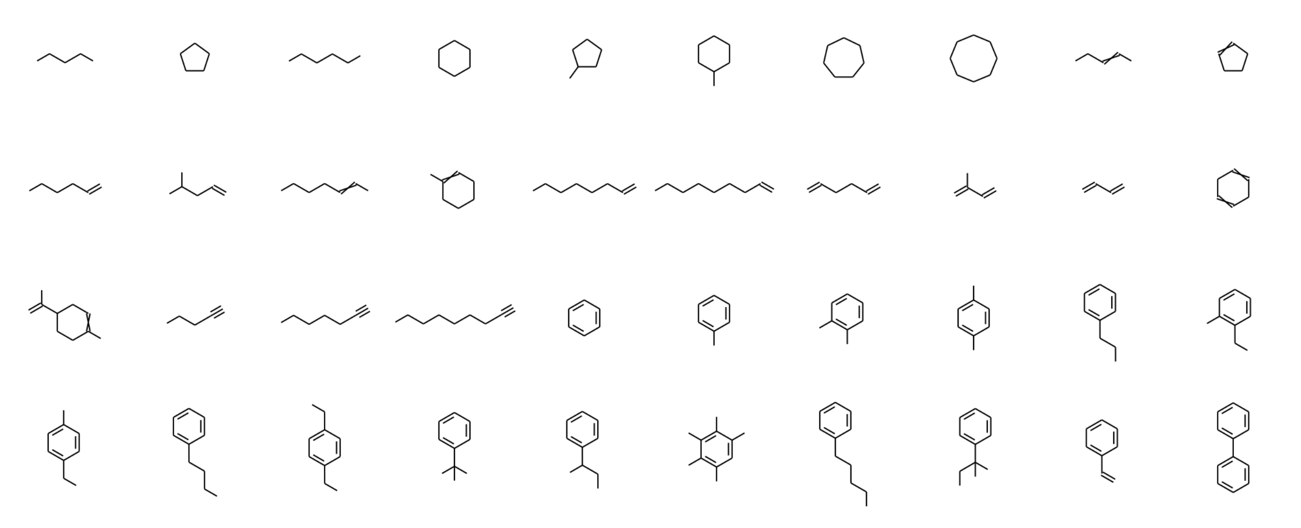
以下のような化合物が含まれています.
2.3 ノード・エッジ特徴量 / 隣接関係の取得
GCNに化学構造を投入するために, 分子中の原子の隣接関係と原子の特徴をベクトル化します.
以下のコードはDeepChemをベースにiwatobipen氏が拡張を行った実装コードです.
以下のmol2graph.pyをPythonファイルとしてインポートして使用してください.
import numpy as np
from rdkit import Chem
import torch
from torch_geometric.data import Data


def one_of_k_encoding(x, allowable_set):
    """
    Encodes elements of a provided set as integers.
    Parameters
     ----------
    x: object
    Must be present in `allowable_set`.
    allowable_set: list
    List of allowable quantities.
    Example
    -------
    >>> import deepchem as dc
    >>> dc.feat.graph_features.one_of_k_encoding("a", ["a", "b", "c"])
    [True, False, False]
    Raises
    ------
    `ValueError` if `x` is not in `allowable_set`.
    """
    if x not in allowable_set:
        raise Exception("input {0} not in allowable set{1}:".format(x, allowable_set))
    return list(map(lambda s: x == s, allowable_set))


def one_of_k_encoding_unk(x, allowable_set):
    """
    Maps inputs not in the allowable set to the last element.
    Unlike `one_of_k_encoding`, if `x` is not in `allowable_set`, this method
    pretends that `x` is the last element of `allowable_set`.
    Parameters
    ----------
    x: object
    Must be present in `allowable_set`.
    allowable_set: list
    List of allowable quantities.
    Examples
    --------
    >>> dc.feat.graph_features.one_of_k_encoding_unk("s", ["a", "b", "c"])
    [False, False, True]
  """
    if x not in allowable_set:
        x = allowable_set[-1]
    return list(map(lambda s: x == s, allowable_set))


def get_intervals(l):
    """For list of lists, gets the cumulative products of the lengths"""
    intervals = len(l) * [0]
    intervals[0] = 1# Initalize with 1
    for k in range(1, len(l)):
        intervals[k] = (len(l[k]) + 1) * intervals[k - 1]
    return intervals


def safe_index(l, e):
    """Gets the index of e in l, providing an index of len(l) if not found"""
    try:
        return l.index(e)
    except:
        return len(l)


class GraphConvConstants(object):
    """This class defines a collection of constants which are useful for graph convolutions on molecules."""
    possible_atom_list = [
          'C', 'N', 'O', 'S', 'F', 'P', 'Cl', 'Mg', 'Na', 'Br', 'Fe', 'Ca', 'Cu','Mc', 'Pd', 'Pb', 'K', 'I', 'Al', 'Ni', 'Mn'
      ]
    """Allowed Numbers of Hydrogens"""
    possible_numH_list = [0, 1, 2, 3, 4]
    """Allowed Valences for Atoms"""
    possible_valence_list = [0, 1, 2, 3, 4, 5, 6]
    """Allowed Formal Charges for Atoms"""
    possible_formal_charge_list = [-3, -2, -1, 0, 1, 2, 3]
    """This is a placeholder for documentation. These will be replaced with corresponding values of the rdkit HybridizationType"""
    possible_hybridization_list = ["SP", "SP2", "SP3", "SP3D", "SP3D2"]
    """Allowed number of radical electrons."""
    possible_number_radical_e_list = [0, 1, 2]
    """Allowed types of Chirality"""
    possible_chirality_list = ['R', 'S']
    """The set of all values allowed."""
    reference_lists = [
          possible_atom_list, possible_numH_list, possible_valence_list,
          possible_formal_charge_list, possible_number_radical_e_list,
          possible_hybridization_list, possible_chirality_list
      ]
    """The number of different values that can be taken. See `get_intervals()`"""
    intervals = get_intervals(reference_lists)
    """Possible stereochemistry. We use E-Z notation for stereochemistry
    https://en.wikipedia.org/wiki/E%E2%80%93Z_notation"""
    possible_bond_stereo = ["STEREONONE", "STEREOANY", "STEREOZ", "STEREOE"]
    """Number of different bond types not counting stereochemistry."""
    bond_fdim_base = 6


def get_feature_list(atom):
    possible_atom_list = GraphConvConstants.possible_atom_list
    possible_numH_list = GraphConvConstants.possible_numH_list
    possible_valence_list = GraphConvConstants.possible_valence_list
    possible_formal_charge_list = GraphConvConstants.possible_formal_charge_list
    possible_number_radical_e_list = GraphConvConstants.possible_number_radical_e_list
    possible_hybridization_list = GraphConvConstants.possible_hybridization_list
    # Replace the hybridization
    from rdkit import Chem
    #global possible_hybridization_list
    possible_hybridization_list = [
        Chem.rdchem.HybridizationType.SP, Chem.rdchem.HybridizationType.SP2,
        Chem.rdchem.HybridizationType.SP3, Chem.rdchem.HybridizationType.SP3D,
        Chem.rdchem.HybridizationType.SP3D2
    ]
    features = 6 * [0]
    features[0] = safe_index(possible_atom_list, atom.GetSymbol())
    features[1] = safe_index(possible_numH_list, atom.GetTotalNumHs())
    features[2] = safe_index(possible_valence_list, atom.GetImplicitValence())
    features[3] = safe_index(possible_formal_charge_list, atom.GetFormalCharge())
    features[4] = safe_index(possible_number_radical_e_list,
                               atom.GetNumRadicalElectrons())
    features[5] = safe_index(possible_hybridization_list, atom.GetHybridization())
    return features


def features_to_id(features, intervals):
    """Convert list of features into index using spacings provided in intervals"""
    id = 0
    for k in range(len(intervals-1)):
        id += features[k] * intervals[k]
    # Allow 0 index to correspond to null molecule 1
    id = id + 1
    return id


def id_to_features(id, intervals):
    features = 6 * [0]
    # Correct for null
    id -= 1
    for k in range(0, 6 - 1):
        # print(6-k-1, id)
        features[6 - k - 1] = id // intervals[6 - k - 1]
        id -= features[6 - k - 1] * intervals[6 - k - 1]
    # Correct for last one
    features[0] = id
    return features


def atom_to_id(atom):
    """Return a unique id corresponding to the atom type"""
    features = get_feature_list(atom)
    return features_to_id(features, intervals)


def atom_features(atom, bool_id_feat=False, explicit_H=False,use_chirality=False):
    if bool_id_feat:
        return np.array([atom_to_id(atom)])
    else:
        # concatnate all atom features
        results_ = one_of_k_encoding_unk(
            atom.GetSymbol(),
            [
                'C',
                'N',
                'O',
                'S',
                'F',
                'Si',
                'P',
                'Cl',
                'Br',
                'Mg',
                'Na',
                'Ca',
                'Fe',
                'As',
                'Al',
                'I',
                'B',
                'V',
                'K',
                'Tl',
                'Yb',
                'Sb',
                'Sn',
                'Ag',
                'Pd',
                'Co',
                'Se',
                'Ti',
                'Zn',
                'H',
                'Li',
                'Ge',
                'Cu',
                'Au',
                'Ni',
                'Cd',
                'In',
                'Mn',
                'Zr',
                'Cr',
                'Pt',
                'Hg',
                'Pb',
                'Unknown'
            ]
        )
        results=results_ + \
        one_of_k_encoding(
            atom.GetDegree(),
            [0, 1, 2, 3, 4, 5, 6, 7, 8, 9, 10]
        ) + \
        one_of_k_encoding_unk(
            atom.GetImplicitValence(),
            [0, 1, 2, 3, 4, 5, 6]
        ) + \
        [
            atom.GetFormalCharge(), atom.GetNumRadicalElectrons()
        ] + \
        one_of_k_encoding_unk(
            atom.GetHybridization().name,
            [
                Chem.rdchem.HybridizationType.SP.name,
                Chem.rdchem.HybridizationType.SP2.name,
                Chem.rdchem.HybridizationType.SP3.name,
                Chem.rdchem.HybridizationType.SP3D.name,
                Chem.rdchem.HybridizationType.SP3D2.name
              ]
            ) + \
        [atom.GetIsAromatic()]
    # In case of explicit hydrogen(QM8, QM9), avoid calling `GetTotalNumHs`
    if not explicit_H:
        results = results + one_of_k_encoding_unk(
            atom.GetTotalNumHs(),
            [0, 1, 2, 3, 4]
        )
    if use_chirality:
        try:
            results = results + one_of_k_encoding_unk(
            atom.GetProp('_CIPCode'),
            ['R', 'S']) + [atom.HasProp('_ChiralityPossible')]
        except:
            results = results + [False, False] + [atom.HasProp('_ChiralityPossible')]

    return np.array(results)


def bond_features(bond, use_chirality=False):
    from rdkit import Chem
    bt = bond.GetBondType()
    bond_feats = [
        bt == Chem.rdchem.BondType.SINGLE, bt == Chem.rdchem.BondType.DOUBLE,
        bt == Chem.rdchem.BondType.TRIPLE, bt == Chem.rdchem.BondType.AROMATIC,
        bond.GetIsConjugated(),
        bond.IsInRing()
    ]
    if use_chirality:
        bond_feats = bond_feats + one_of_k_encoding_unk(
            str(bond.GetStereo()),
            ["STEREONONE", "STEREOANY", "STEREOZ", "STEREOE"]
        )
    return np.array(bond_feats)

def get_bond_pair(mol):
    bonds = mol.GetBonds()
    res = [[],[]]
    for bond in bonds:
        res[0] += [bond.GetBeginAtomIdx(), bond.GetEndAtomIdx()]
        res[1] += [bond.GetEndAtomIdx(), bond.GetBeginAtomIdx()]
    return res

def mol2vec(mol):
    atoms = mol.GetAtoms()
    bonds = mol.GetBonds()
    node_f= [atom_features(atom) for atom in atoms]
    edge_index = get_bond_pair(mol)
    edge_attr = [bond_features(bond, use_chirality=False) for bond in bonds]
    for bond in bonds:
        edge_attr.append(bond_features(bond))
        data = Data(
            x=torch.tensor(node_f, dtype=torch.float), # shape [num_nodes, num_node_features] を持つ特徴行列
            edge_index=torch.tensor(edge_index, dtype=torch.long), #shape [2, num_edges] と型 torch.long を持つ COO フォーマットによるグラフ連結度
            edge_attr=torch.tensor(edge_attr,dtype=torch.float) # shape [num_edges, num_edge_features] によるエッジ特徴行列
        )
    return data
ソースコードは長いですが, 要点はシンプルです.
PyTorch geometricのGCNConvを機能させるために必要な入力情報は以下の3つです.
-
グラフ内の全ての頂点の特徴ベクトルを含んだ行列
x=torch.tensor(node_f, dtype=torch.float)の部分です.
ここには[num_nodes, num_node_features]のshapeを持つ特徴行列が入ります.
node_featuresには原子種, 混成軌道の種類, 水素数などが用いられ, これらの情報をone-hot-voctor化したものが原子の有する特徴ベクトルとなります. -
エッジが結ぶ頂点のペアを指定した行列
edge_index=torch.tensor(edge_index, dtype=torch.long)の部分です.
[2, num_edges] のshapeを持ちそれぞれのエッジがどの頂点とリンクしているかを情報として持ちます. -
エッジの特徴ベクトルを格納した行列
edge_attr=torch.tensor(edge_attr,dtype=torch.float)の部分です.
[num_edges, num_edge_features]のshapeを持つ特徴行列が入ります.
edge_featuresには単結合, 二重結合, 三重結合, 芳香族結合などの情報が用いられ, これらの情報をone-hot-voctor化したものがエッジの有する特徴ベクトルとなります.
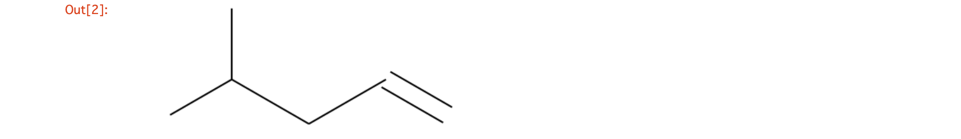
例
from rdkit import Chem
mols = [mol for mol in Chem.SDMolSupplier('solubility.train.sdf')]
mol = mols[15]
atoms = mol.GetAtoms()
mol
DeepChemの実装ではグラフから原子の特徴を抽出するとき以下の7要素を考慮し, これらをohe-hot-vector化することで1原子あたり75次元の特徴ベクトルを取得します
print('Atomic symbol type')
print([atom.GetSymbol() for atom in atoms])
print('The number of adjacent atoms')
print([atom.GetDegree() for atom in atoms])
print('The number of hydrodens')
print([atom.GetTotalNumHs() for atom in atoms])
print('Maximum number of possible connections')
print([atom.GetImplicitValence() for atom in atoms])
print('From charges')
print([atom.GetFormalCharge() for atom in atoms])
print('The number of radical electrons')
print([atom.GetNumRadicalElectrons() for atom in atoms])
print('The type of hybrid orbit')
print([atom.GetHybridization() for atom in atoms])
Atomic symbol type
['C', 'C', 'C', 'C', 'C', 'C']
The number of adjacent atoms
[1, 3, 1, 2, 2, 1]
The number of hydrodens
[3, 1, 3, 2, 1, 2]
Maximum number of possible connections
[3, 1, 3, 2, 1, 2]
From charges
[0, 0, 0, 0, 0, 0]
The number of radical electrons
[0, 0, 0, 0, 0, 0]
The type of hybrid orbit
[rdkit.Chem.rdchem.HybridizationType.SP3, rdkit.Chem.rdchem.HybridizationType.SP3, rdkit.Chem.rdchem.HybridizationType.SP3, rdkit.Chem.rdchem.HybridizationType.SP3, rdkit.Chem.rdchem.HybridizationType.SP2, rdkit.Chem.rdchem.HybridizationType.SP2]
2.4 GCNの学習と予測
import numpy as np
import matplotlib.pyplot as plt
from sklearn.model_selection import KFold
from sklearn.metrics import mean_squared_error, r2_score

from rdkit import Chem
from rdkit.Chem import Draw

import torch
import torch.nn.functional as F
from torch.nn import ModuleList, Linear, BatchNorm1d
from torch_geometric.nn import GCNConv
from torch_geometric.nn import global_add_pool, global_mean_pool
from torch_geometric.data import DataLoader

import mol2graph

# Device settings
if torch.cuda.is_available():
    device = torch.device('cuda')
    print('The code uses GPU!')
else:
    device = torch.device('cpu')
    print('The code uses CPU...')

# Load dataset
mols = np.array([mol for mol in Chem.SDMolSupplier('solubility.train.sdf')])
proparties = np.array([mol.GetProp('SOL') for mol in mols], dtype=float)

kf = KFold(n_splits=5, random_state=1640, shuffle=True)
train_idx, test_idx = list(kf.split(mols, np.zeros(len(mols))))[0]
train_X = [mol2graph.mol2vec(m) for m in mols[train_idx].tolist()]
train_y = proparties[train_idx]
for i, data in enumerate(train_X):
    data.y = torch.FloatTensor([train_y[i]]).to(device)
test_X = [mol2graph.mol2vec(m) for m in mols[test_idx].tolist()]
test_y = proparties[test_idx]
for i, data in enumerate(test_X):
    data.y = torch.FloatTensor([test_y[i]]).to(device)

train_loader = DataLoader(train_X, batch_size=64, shuffle=True, drop_last=True)
test_loader = DataLoader(test_X, batch_size=64, shuffle=True, drop_last=True)


# Molecular GCN
class MolecularGCN(torch.nn.Module):
    def __init__(self):
        super(MolecularGCN, self).__init__()
        self.n_features = 75 #  This is the mol2graph.py-specific value
        self.n_conv_hidden = 3
        self.n_mlp_hidden = 3
        self.dim = 64
        self.graphconv1 = GCNConv(self.n_features, self.dim)
        self.bn1 = BatchNorm1d(self.dim)
        self.graphconv_hidden = ModuleList(
            [GCNConv(self.dim, self.dim, cached=False) for _ in range(self.n_conv_hidden)]
        )
        self.bn_conv = ModuleList(
            [BatchNorm1d(self.dim) for _ in range(self.n_conv_hidden)]
        )
        self.mlp_hidden =  ModuleList(
            [Linear(self.dim, self.dim) for _ in range(self.n_mlp_hidden)]
        )
        self.bn_mlp = ModuleList(
            [BatchNorm1d(self.dim) for _ in range(self.n_mlp_hidden)]
        )
        self.mlp_out = Linear(self.dim,1)

    def forward(self, data):
        x, edge_index = data.x, data.edge_index
        x = F.relu(self.graphconv1(x, edge_index))
        x = self.bn1(x)
        for graphconv, bn_conv in zip(self.graphconv_hidden, self.bn_conv):
            x = graphconv(x, edge_index)
            x = bn_conv(x)
        x = global_add_pool(x, data.batch)
        for fc_mlp, bn_mlp in zip(self.mlp_hidden, self.bn_mlp):
            x = F.relu(fc_mlp(x))
            x = bn_mlp(x)
            x = F.dropout(x, p=0.1, training=self.training)
        x = self.mlp_out(x)
        return x


# Trainning and prediction
model = MolecularGCN().to(device)
optimizer = torch.optim.Adam(model.parameters(), lr=0.001)

def train(epoch):
    model.train()
    loss_all = 0
    for data in train_loader:
        data = data.to(device)
        optimizer.zero_grad()
        output = model(data)
        loss = F.mse_loss(output, data.y.unsqueeze(1))
        loss.backward()
        loss_all += loss.item() * data.num_graphs
        optimizer.step()
    return loss_all / len(train_X)

def test(loader):
    model.eval()
    P, T, R2 = [], [], []
    for data in loader:
        data = data.to(device)
        y_pred = model(data)
        P.append(y_pred.detach().numpy())
        T.append(data.y.detach().numpy())
        R2.append(r2_score(y_pred.detach().numpy(), data.y.detach().numpy()))
    return  np.concatenate(T), np.concatenate(P), np.mean(R2)

hist = {
    "mae":[],
    "r2":[],
    "test_r2":[],
    'y_true_train':[],
    'y_pred_train':[],
    'y_true_test':[],
    'y_pred_test':[],
}

for epoch in range(1, 200):
    train_mse = train(epoch)
    y_train, y_train_pred, train_r2 = test(train_loader)
    y_test, y_test_pred, test_r2 = test(test_loader)
    hist["mae"].append(train_mse)
    hist["r2"].append(train_r2)
    hist["test_r2"].append(test_r2)
    hist['y_true_train'].append(y_train)
    hist['y_pred_train'].append(y_train_pred)
    hist['y_true_test'].append(y_test)
    hist['y_pred_test'].append(y_test_pred)
    print(f'Epoch: {epoch}, Train MAE: {train_mse:.3}, Train_R2: {train_r2:.3}, Test_R2: {test_r2:.3}')
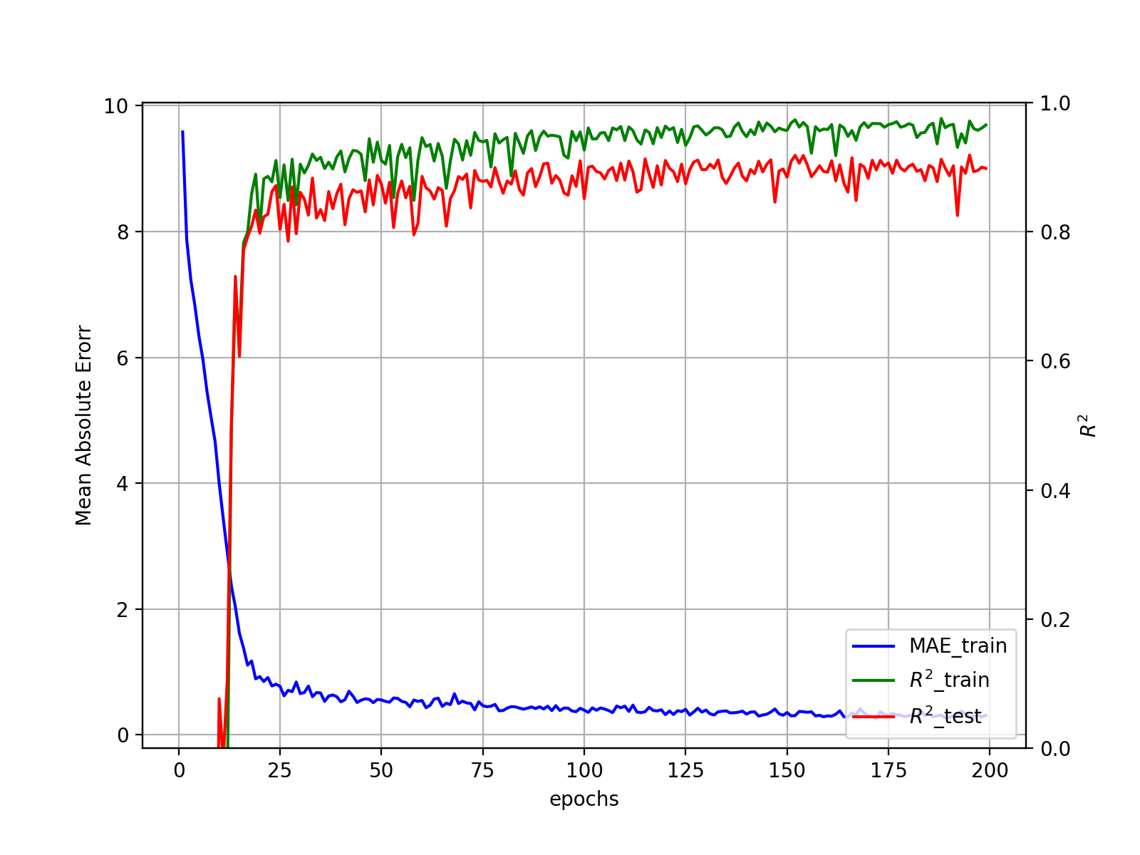
学習過程を可視化します
fig = plt.figure(figsize=(8,6))
ax1 = fig.add_subplot(111)
ax2 = ax1.twinx()
epochs = np.arange(1,200)
ax1.plot(epochs, hist['mae'], label="MAE_train", c='blue')
ax2.plot(epochs, hist['r2'], label=r"$R^2$_train", c='green')
ax2.plot(epochs, hist['test_r2'], label=r"$R^2$_test", c='red')
ax1.set_xlabel('epochs')
ax1.set_ylabel(r'Mean Absolute Erorr')
ax1.grid(True)
ax2.set_ylabel(r'$R^2$')
ax2.set_ylim([0,1])
h1, l1 = ax1.get_legend_handles_labels()
h2, l2 = ax2.get_legend_handles_labels()
ax1.legend(h1+h2, l1+l2, loc='lower right')
plt.show()
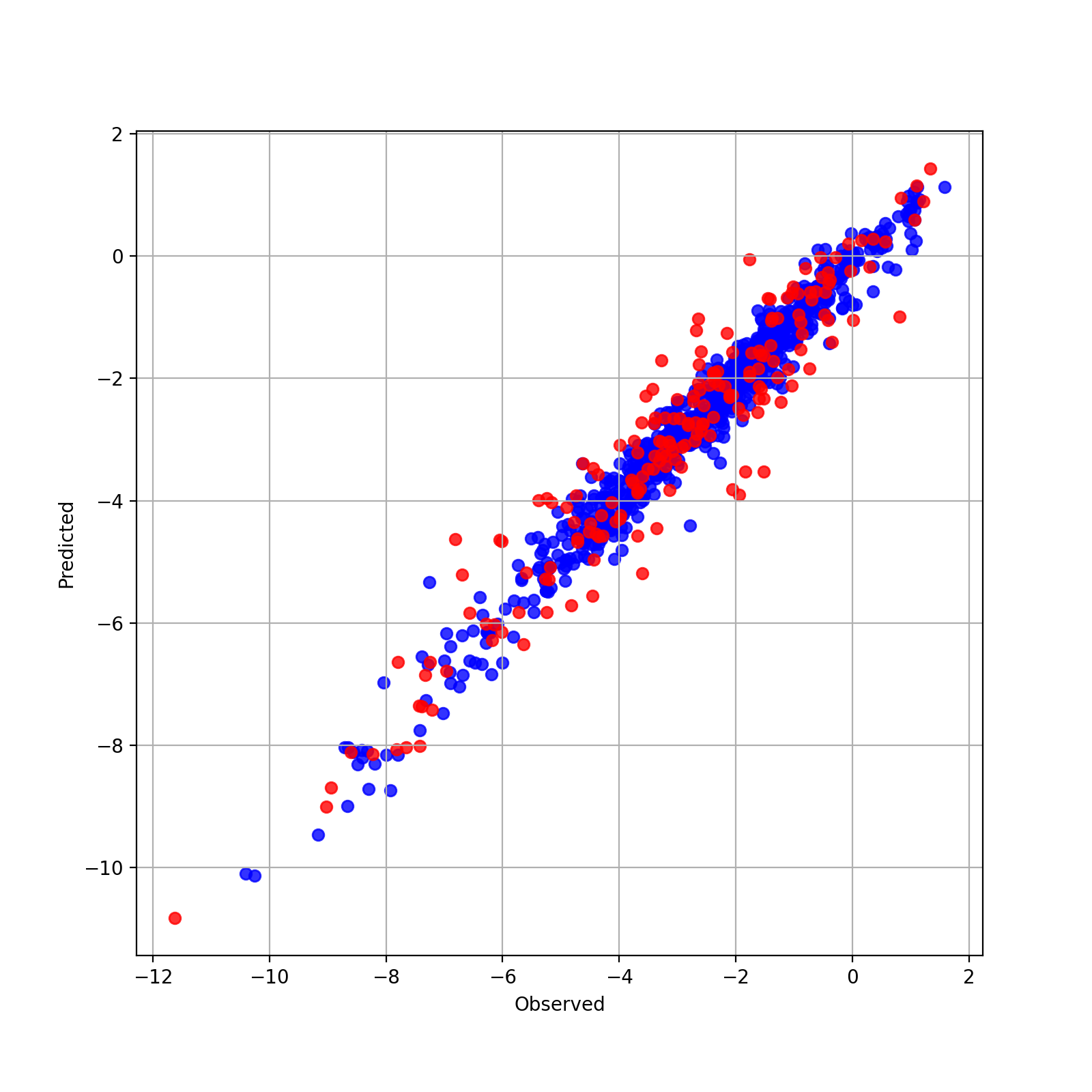
実測値と予測値の散布図を表示してみましょう.
plt.figure(figsize=(8,8))
plt.grid(True)
plt.scatter(hist['y_true_train'][-1], hist['y_pred_train'][-1], color='blue', alpha=0.8, label='train')
plt.scatter(hist['y_true_test'][-1], hist['y_pred_test'][-1], color='red', alpha=0.8, label='test')
plt.ylabel("Predicted")
plt.xlabel("Observed")
plt.legend()