HuggingFace(BERT)を便利なTrainerを使用して分類する

0. はじめに

最近HuggingFaceを使う時に、Trainerを使うと便利なことがわかったので本記事は自分へのメモ用として残しておく
※以下記事はvalidが無かったりする為、本記事は改訂版の位置づけともなっている
※あえて本記事では自作でmodel部分をカスタマイズさせたりしている

★本記事の全コードをGoogle Colabでも共有しました

• 動作環境
  • OS : Windows10 pro
  • python： 3.9.6　
  • transformers： 4.23.1
  • Pytorch： 1.12.1 (+cu116)
  • jupyter notebook(vscode)

まずは本記事で使用するライブラリ群のインポートとseed固定を最初に書いておく。

ライブラリimport＋seed固定

#本記事で使うライブラリ群
import os
import random
import warnings
warnings.simplefilter('ignore')

import pandas as pd
import numpy as np

import transformers
from transformers import (
    AutoModel, AutoTokenizer, EvalPrediction, Trainer,
    TrainingArguments, AutoModelForSequenceClassification,
    EarlyStoppingCallback,
)
from transformers.modeling_outputs import SequenceClassifierOutput
from transformers import BertPreTrainedModel, BertModel

import torch
import torch.nn as nn

from sklearn.model_selection import train_test_split
from sklearn.metrics import f1_score

from torch.utils.data import Dataset
from sklearn.metrics import accuracy_score, precision_recall_fscore_support

from torchinfo import summary

#乱数固定
def seed_everything(seed: int):
    """seed固定"""
    random.seed(seed)
    os.environ['PYTHONHASHSEED'] = str(seed)
    np.random.seed(seed)
    torch.manual_seed(seed)
    torch.cuda.manual_seed(seed)
    torch.backends.cudnn.deterministic = True
    torch.backends.cudnn.benchmark = True

SEED = 7
seed_everything(SEED)

1. livedoor ニュースコーパスをデータフレームにする

ここら辺の準備等の詳細は前回記事に詳しく書いたので参照ください。

本jupyterの実行ディレクトリにlivdoor_dataというフォルダを用意し、その中にDLしたコーパスを入れてます。

ニュースコーパスをデータフレーム化

def get_title_list(path):
    """記事タイトル取得関数"""
    title_list = []
    filenames = os.listdir(path) #ファイル名称一覧取得
    for filename in filenames:
        # 1記事ずつファイルの読み込み
        with open(path+filename, encoding="utf_8_sig") as f:
            title = f.readlines()[2].strip()
            title_list.append(title)
    return title_list

#コーパスをDLして格納したディレクトリ
DATA_DIR = "./livdoor_data"

#空データフレームを用意
df = pd.DataFrame(columns=['label', 'sentence'])

#用意した空データフレームにappendしていく
#独女通信(ラベル0)
title_list = get_title_list(DATA_DIR + '/dokujo-tsushin/')
for title in title_list:
    df = df.append({'label':0 , 'sentence':title}, ignore_index=True)
#ITライフハック(ラベル1)
title_list = get_title_list(DATA_DIR + '/it-life-hack/')
for title in title_list:
    df = df.append({'label':1 , 'sentence':title}, ignore_index=True)
#MOVIE ENTER(ラベル2)
title_list = get_title_list(DATA_DIR + '/movie-enter/')
for title in title_list:
    df = df.append({'label':2 , 'sentence':title}, ignore_index=True)

# 全データの順番をシャッフル(+index振り直し)
df = df.sample(frac=1 ,random_state=0).reset_index(drop=True)

#お試しで2行表示
df.head(2)

	label	sentence
0	1	楽しくリズム感覚が身につく「おやこでリズムえほんプラス」【iPhoneでチャンスを掴め】
1	2	懐かしのゲームブックをネットで再現 「鷹の団のガッツになってドルドレイを攻略せよ！」

2. train/val/testに分割

train_test_splitだと2回書かないといけないので、numpy.splitを使って1行で書く

#参考：https://stmind.hatenablog.com/entry/2022/03/12/165426

train/val/testに分割

#最初の6割をtrain、次の2割をvalid、最後の2割をtestでデータフレームを分割
train, val, test = np.split(df, [int(len(df) * .6), int(len(df) * .8)])

print(train.shape)
print(val.shape)
print(test.shape)
#お試しで1行ずつ表示
display(train.head(1))
display(val.head(1))
display(test.head(1))

実行結果

(1567, 2)
(523, 2)
(523, 2)

	label	sentence
0	1	楽しくリズム感覚が身につく「おやこでリズムえほんプラス」【iPhoneでチャンスを掴め】

	label	sentence
1567	0	独身男性は独女より人妻と遊びたいってホント？

	label	sentence
2090	0	独女世代が気になる女の条件とは

3. tokenizer

tokenizerを指定する。今回もbert-base-japanese-v2を使用する。
ここも詳細やイメージは前回記事を参照のこと

トークナイザを指定

MODEL_NAME = "cl-tohoku/bert-base-japanese-v2"

#東北大Wikipediaモデルの2020年8月実行＋BERT-Baseモデル版を指定
tokenizer = AutoTokenizer.from_pretrained(pretrained_model_name_or_path = MODEL_NAME)

ids = tokenizer.encode(train['sentence'][0])
wakati = tokenizer.convert_ids_to_tokens(ids)
print(train['sentence'][0])
print(ids)
print(wakati)

実行結果

楽しくリズム感覚が身につく「おやこでリズムえほんプラス」【iPhoneでチャンスを掴め】
[2, 32589, 17651, 16947, 862, 5128, 893, 12953, 838, 25413, 6550, 889, 17651, 858, 20063, 14384, 839, 842, 28029, 889, 18394, 932, 2592, 6381, 843, 3]
['[CLS]', '楽しく', 'リズム', '感覚', 'が', '身', 'に', 'つく', '「', 'おや', '##こ', 'で', 'リズム', 'え', '##ほん', 'プラス', '」', '【', 'iPhone', 'で', 'チャンス', 'を', '掴', '##め', '】', '[SEP]']

4. BERTのmodel定義

前回記事では、BertForSequenceClassification(AutoModelForSequenceClassification)を使用していたので、今回はあえて自分でClassを書いてみる。
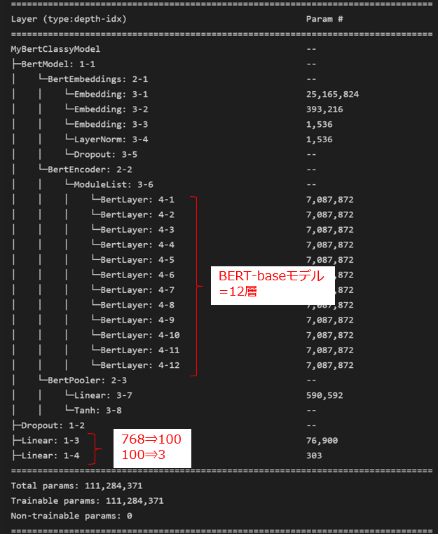
BertForTokenClassificationと同じではつまらないので、BERTのベクトル768次元からいくなり分類数の次元に圧縮するのではなく、間に100次元への次元圧縮を加えたパターンとした。

※ 公式のBertForTokenClassificationクラスを参考に自己流で書いているのであくまで参考程度で。。。

BERTを定義し、modelとして登録する

class MyBertClassyModel(BertPreTrainedModel):
    def __init__(self, config):
        super().__init__(config)
        self.num_labels = config.num_labels
        self.config = config
        self.bert = BertModel(config)
        #以下は線形部分。768から一気に3次元(分類数=3)にせずに100次元を追加
        self.dropout = nn.Dropout(0.5)
        self.linear1 = nn.Linear(768, 100) # 768⇒100
        self.linear2 = nn.Linear(100, 3) # 100⇒3
        
    def forward(self, input_ids=None, attention_mask=None, token_type_ids=None\
        , labels=None, output_attentions=None, output_hidden_states=None):
        #BERTで768次元のベクトルを出力
        outputs = self.bert(
            input_ids, 
            attention_mask=attention_mask,
            token_type_ids=token_type_ids
        )
        #線形変換し、最終的には3次元まで次元削減する
        outputs = self.dropout(outputs.last_hidden_state[:, 0, :])
        outputs = self.linear1(outputs) # 768⇒100
        outputs = self.linear2(outputs) # 100⇒3
        
        loss = None
        if labels is not None:
            loss_fct = nn.CrossEntropyLoss()
            loss = loss_fct(outputs.view(-1, self.num_labels), labels.view(-1))
        
        #SequenceClassifierOutputは文章分類用のデータクラス
        return  SequenceClassifierOutput(
            loss=loss,
            logits=outputs,
            hidden_states=output_hidden_states,
            attentions=output_attentions,
        )

# モデルのインスタンス化
model = MyBertClassyModel.from_pretrained(MODEL_NAME, num_labels=3)

#簡単にやりたいならわざわざ自分でclass定義せずに以下だけでOK
# model = AutoModelForSequenceClassification.from_pretrained(MODEL_NAME, num_labels = 3)

# torchinfoで中身を確認
summary(model, depth=4)

★torchinfoの出力

5. BERTモデルの勾配更新させる場所を指定する

これも別にやらなくていいが、せっかくなので1つのサンプルとして残しておく。
通常のファインチューニングでは「BERTレイヤー」含めチューニング対象に合わせて最適化するが、今回はあえて「BERTの最後の部分＋線形」部分だけ勾配更新させるように記載する。　
※このライブドアのお題ではこの項目をやった方が精度低くなります
よって不要ならこの「5. 勾配更新させる場所を指定する」はまるごと飛ばして次「6. データセット作成」へ進んでもOKです

勾配更新箇所を限定する

#まずは定義したmodelの全層の購買を更新させなくする ※print(name)で層の名称を確認可能
for name, param in model.named_parameters():
    # print(name)
    param.requires_grad = False

#BERTの最終層「self.bertのencoder層ラスト(-1)」だけ勾配更新するようにする
for name, param in model.bert.encoder.layer[-1].named_parameters():
    param.requires_grad = True

#さらに、自分で定義したモデルの「全結合層(self.linear1/self.linear2)」だけ勾配更新するようにする
for name, param in model.linear1.named_parameters():
    param.requires_grad = True
for name, param in model.linear2.named_parameters():
    param.requires_grad = True

#最後に勾配更新対象の層を確認する
for name, param in model.named_parameters():
    if param.requires_grad : print(name)

すると、BERTの最終層(0スタートなので11層目)と線形部分だけ表示されるはず

実行結果

bert.encoder.layer.11.attention.self.query.weight
bert.encoder.layer.11.attention.self.query.bias
bert.encoder.layer.11.attention.self.key.weight
bert.encoder.layer.11.attention.self.key.bias
bert.encoder.layer.11.attention.self.value.weight
bert.encoder.layer.11.attention.self.value.bias
bert.encoder.layer.11.attention.output.dense.weight
bert.encoder.layer.11.attention.output.dense.bias
bert.encoder.layer.11.attention.output.LayerNorm.weight
bert.encoder.layer.11.attention.output.LayerNorm.bias
bert.encoder.layer.11.intermediate.dense.weight
bert.encoder.layer.11.intermediate.dense.bias
bert.encoder.layer.11.output.dense.weight
bert.encoder.layer.11.output.dense.bias
bert.encoder.layer.11.output.LayerNorm.weight
bert.encoder.layer.11.output.LayerNorm.bias
linear1.weight
linear1.bias
linear2.weight
linear2.bias

6. データセット作成

まずは最大トークン数を調べ、次にtrain/val/testのinput部分を作成する

train/val/testのinput部分作成

#全データのトークン数をlist化しておく
text_lengths_list = [len(tokenizer.encode(text)) for text in df["sentence"].to_list()]

#データセットにinputさせるトークナイザ部分を定義
"""
padding="max_length"にすることで、max_lengthで指定(最大トークン数)した長さのトークン分paddingしてくれる
前回記事の記載のようにpadding=Trueだとtrainの中しか見ないので注意。
"""
train_X = [tokenizer(text, padding="max_length", max_length=max(text_lengths_list), truncation=True) for text in train["sentence"]]
valid_X = [tokenizer(text, padding="max_length", max_length=max(text_lengths_list), truncation=True) for text in val["sentence"]]
test_X = [tokenizer(text, padding="max_length", max_length=max(text_lengths_list), truncation=True) for text in test["sentence"]]

#お試し表示
print(f"最大トークン数は{max(text_lengths_list)}です")
print(train_X.keys())
print(len(train_X['input_ids']))
print(len(valid_X['input_ids']))
print(len(test_X['input_ids']))

実行結果

最大トークン数は47です
dict_keys(['input_ids', 'token_type_ids', 'attention_mask'])
1567
523
523

後はデータセットを作成する

データセットを定義し、作成

class MyDataset(Dataset):
  def __init__(self, encodings, labels=None):
    self.encodings = encodings
    self.labels = labels

  def __len__(self):
    return len(self.encodings['input_ids'])

  def __getitem__(self, index):
    input = {key: torch.tensor(val[index]) for key, val in self.encodings.items()}
    if self.labels is not None:
        input["label"] = torch.tensor(self.labels[index])

    return input

#train/valid/testのデータセットをそれぞれ作成する ※testは当然label無し
train_ds = MyDataset(train_X, train["label"].tolist())
valid_ds = MyDataset(valid_X, val["label"].tolist())
test_ds = MyDataset(test_X)

#お試し確認
print(train_ds[0].keys())
print(f"学習データ数は{len(train_ds)}です")
print(tokenizer.decode(train_ds[0]["input_ids"])) #デコードで戻してみる

実行結果

dict_keys(['input_ids', 'token_type_ids', 'attention_mask', 'label'])
学習データ数は1567です
[CLS] 楽しく リズム 感覚 が 身 に つく 「 おやこ で リズム えほん プラス 」 【 iPhone で チャンス を 掴め 】 [SEP] 
[PAD] [PAD] [PAD] [PAD] [PAD] [PAD] [PAD] [PAD] [PAD] [PAD] [PAD] [PAD] [PAD] [PAD] [PAD] [PAD] [PAD] [PAD] 
[PAD] [PAD] [PAD]

7. trainerで学習

さて、ようやく本記事の本題である。
ただ以下に詳細が書いてあるので、説明は最低限としかなり端折っていく。

7-1. compute_metrics

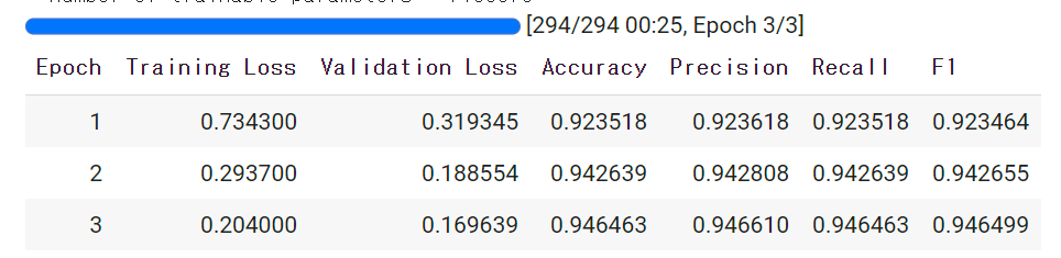
ここでは、Trainerに渡す評価指標を定義する。
なお、これを省略した場合には結果がlogにしか記載されないらしい。
下記コードではsklearnのprecision_recall_fscore_supportで各種指標を計算し、accを加えている。
私の環境(vscodeのjupyter)では少し表示がおかしいが、Google Colabや通常のjupyterではLOGとしてここで設定した項目が出力される。

compute_metrics

def compute_metrics(pred):
    labels = pred.label_ids
    preds = pred.predictions.argmax(-1)
    #2値分類ならaverage='binary'とする
    precision, recall, f1, _ = precision_recall_fscore_support(labels, preds, average='weighted', zero_division=0)
    acc = accuracy_score(labels, preds)
    return {
        'accuracy': acc,
        'precision': precision,
        'recall': recall,
        'f1': f1,
    }

★ここで定義したものが以下のように(LOSSに加えて)出力される。(出力はtrainer.train()で行われます)

7-2. TrainingArguments

ここではTrainerに渡す設定を記載する。
全部説明すると無茶苦茶多いので、詳細は公式ドキュメント参照のこと

TrainingArguments

train_args = TrainingArguments(
    output_dir                  = "./out", #log出力場所
    overwrite_output_dir        = True, #logを上書きするか
    load_best_model_at_end      = True, #EarlyStoppingを使用するならTrue
    metric_for_best_model       = "f1", #EarlyStoppingの判断基準。7-1. compute_metricsのものを指定
    save_total_limit            = 1, #output_dirに残すチェックポイントの数
    save_strategy               = "epoch", #いつ保存するか？
    evaluation_strategy         = "epoch", #いつ評価するか？
    logging_strategy            = "epoch", #いつLOGに残すか？
    label_names                 = ['labels'], #分類ラベルのkey名称(デフォルトはlabelsなので注意)
    lr_scheduler_type           = "linear", #学習率の減衰設定(デフォルトlinearなので設定不要)
    learning_rate               = 5e-5, #学習率(デフォルトは5e-5)
    num_train_epochs            = 3, #epoch数
    per_device_train_batch_size = 16, #学習のバッチサイズ
    per_device_eval_batch_size  = 12, #バリデーション/テストのバッチサイズ
    seed                        = SEED, #seed
)

※lr_scheduler_typeは以下に記載あるものが指定可能。
https://huggingface.co/docs/transformers/v4.24.0/en/main_classes/optimizer_schedules#transformers.SchedulerType

なお、この実行後にprint(train_args.device)とすればわかるが、GPUが使える環境なら勝手にGPUがセットされるらしく、
Pytorchでおなじみのmodel.to('cuda')等は別に不要となっているみたい。
※実際にこのサンプルコードではやってないがGPU使われる

7-3. callback

学習中に行いたい処理をここに書いておき、Trainerに渡すことが出来る。
よく使われる例としてEarlyStoppingがあるので、その例を書いておく

callback

#early_stopping_patienceでこの回数スコア(metric_for_best_modelで指定したやつ)更新しないと強制終了。
MyCallback = EarlyStoppingCallback(early_stopping_patience=3)

7-3. Trainerで学習

今まで書いてきたものを指定することで学習可能。

Trainerで学習

trainer = Trainer(
    model=model, #モデル
    args=train_args, #TrainingArguments
    tokenizer=tokenizer, #tokenizer
    train_dataset=train_ds, #学習データセット
    eval_dataset=valid_ds, #validデータセット
    compute_metrics = compute_metrics, #compute_metrics
    callbacks=[MyCallback] #callback
)

trainer.train()

8. trainerでテスト

さて、今回は学習に未使用でラベルが入ってないテスト用データセット(test_ds)を評価させる。

trainerでテスト

#trainer.predictで評価可能
test_preds = trainer.predict(test_ds)

#元のtestデータフレームにpredカラムを追記する
test['pred'] = np.argmax(test_preds.predictions, axis=1)

#評価用にそれぞれ計算し、print
precision, recall, f1_score, _ = precision_recall_fscore_support(test['label'], test['pred'], average=None)
print('正答率（Accuracy） = {:.3f}%'.format(100 * accuracy_score(test['label'], test['pred']))) # 正答率を表示
print('適合率（Precision） = {:.3f}%'.format(100 * precision[0])) # 適合率を表示
print('再現率（Recall） = {:.3f}%'.format(100 * recall[0])) # 再現率を表示
print('F1値（F1-score） = {:.3f}%'.format(100 * f1_score[0])) #F1値を表示

#dfもお試し表示
display(test.head(2))

実行結果

正答率（Accuracy） = 93.117%
適合率（Precision） = 90.698%
再現率（Recall） = 92.308%
F1値（F1-score） = 91.496%

	label	sentence	pred
2090	0	独女世代が気になる女の条件とは	0
2091	2	インタビュー：斉藤和義「音楽バカのカッコ良さを喰らいやがれ！」	2

seabornで可視化

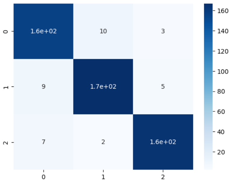
from sklearn.metrics import confusion_matrix
import seaborn as sns

cm = confusion_matrix(test['label'], test['pred'])

sns.heatmap(cm, annot=True, cmap='Blues')

9. (おまけ)pipelineでも結果を見てみる

推論を実行する場合に便利なpipelineもお試ししてみたのでおまけで。
詳細は公式ドキュメントを参照のこと

pipelineで評価

from transformers import pipeline

device = "cuda:0" if torch.cuda.is_available() else "cpu"
#text-classificationではsentiment-analysisを指定するらしい
sentiment_analyzer = pipeline("sentiment-analysis", model=model, tokenizer=tokenizer, device=device)

#大元のdfでもいいし、testデータフレームでもいいがpipelineでも結果確認可能
n=2090
print(test['sentence'][n])
print(f"正解ラベルは{test['label'][n]}です")
print(f"モデルの予測は{sentiment_analyzer(test['sentence'][n])}です")
print('- - -')
print(df['sentence'][n])
print(f"正解ラベルは{df['label'][n]}です")
print(f"モデルの予測は{sentiment_analyzer(df['sentence'][n])}です")

実行結果

独女世代が気になる女の条件とは
正解ラベルは0です
モデルの予測は[{'label': 'LABEL_0', 'score': 0.9778923392295837}]です
- - -
独女世代が気になる女の条件とは
正解ラベルは0です
モデルの予測は[{'label': 'LABEL_0', 'score': 0.9778923392295837}]です

10. おわりに

さて、自分が後で見返しても使えるようにわかりやすく書いたつもりなので参考になっていただけると幸いである。
HuggingFaceで学習させるときは私も今後はこのTrainerを積極的に使うようにしようと思う

また、本記事の全コードをGoogle Colabでも共有しました。(慣れてなくて少し変かも？＋本記事と一部違いはあります)
そちらも参考ください。(コメント少ないので、理解は本記事で・・)