librosaを使った音声データの分析事例

1.はじめに

librosaを利用して、音声データを分析する内容をご紹介します。

2.音声データの理解

y: 振幅データ 、リストとして返される。
sr: Sampling rate [Hz]

import librosa

y, sr = librosa.load('Data/genres_original/rock/rock.00001.wav')
print(y)
print(len(y))
print('Sampling rate (Hz): %d' % sr)
print('Audio length (seconds): %.2f' % (len(y) / sr))

[0.36239624 0.6494751  0.6317444  ... 0.04336548 0.0557251  0.05700684]
661794
Sampling rate (Hz): 22050
Audio length (seconds): 30.01

音楽を聴く

import IPython.display as ipd
ipd.Audio(y, rate=sr)

3.音声データのEDM

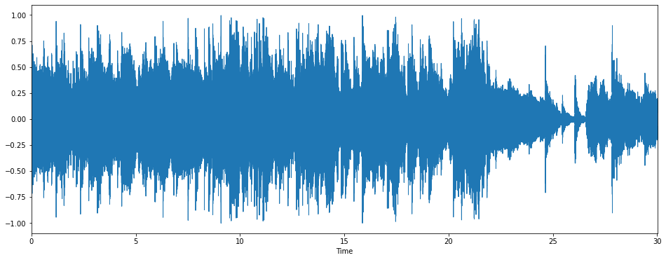
3.1.時間領域のグラフ

import matplotlib.pyplot as plt
import librosa.display

plt.figure(figsize=(16,6))
librosa.display.waveplot(y=y, sr=sr)
plt.show()

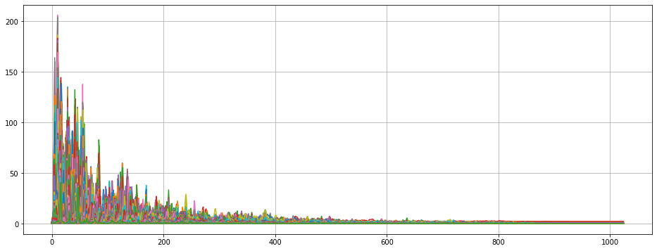
3.2.周波数領域でのグラフ

フーリエ変換を行います。
縦軸：周波数の振幅（ログスケール）
横軸：周波数[Hz]

import numpy as np

D = np.abs(librosa.stft(y, n_fft=2048, hop_length=512))
print(D.shape)

plt.figure(figsize=(16, 6))
plt.plot(D)
plt.grid()
plt.show()

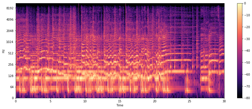
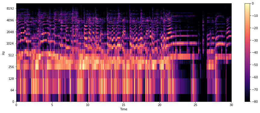
3.3.Spectrogram

時間 vs.　周波数
別称：Sonographs, Voiceprints, Voicegrams

DB = librosa.amplitude_to_db(D, ref=np.max)

plt.figure(figsize=(16, 6))
librosa.display.specshow(DB, sr=sr, hop_length=512, x_axis='time', y_axis='log')
plt.colorbar()
plt.show()

3.4.Mel Spectrogram

Spectrogramの縦軸を人間が理解しやすいMel Scleに変換したもの
非線形変換

S = librosa.feature.melspectrogram(y, sr=sr)
S_DB = librosa.amplitude_to_db(S, ref=np.max)
plt.figure(figsize=(16, 6))
librosa.display.specshow(S_DB, sr=sr, hop_length=512, x_axis='time', y_axis='log')
plt.colorbar()
plt.show()

4.音声データの特徴量の抽出

4.1.Tempo(BPM)

#Tempo

tempo, _ = librosa.beat.beat_track(y, sr=sr)
print(tempo)

151.99908088235293

4.2.Zero Crossing Rate

Zero Crossing Rateは、音声の波形を描いたとき、波が中央より上(正)から中央より下(負)に、またはその逆に変化する頻度を数えて、その頻度により音声の特徴を表すというもの。ZCRが大きいほどより noisy な音声と捉えられるらしい。（下記のページから転載）
http://egawata.hatenablog.com/entry/20140508/1399574234#:~:text=%E9%9F%B3%E5%A3%B0%E8%AA%8D%E8%AD%98%E3%82%84%E9%9F%B3%E6%A5%BD%E8%A7%A3%E6%9E%90,%E7%89%B9%E5%BE%B4%E3%82%92%E8%A1%A8%E3%81%99%E3%81%A8%E3%81%84%E3%81%86%E3%82%82%E3%81%AE%E3%80%82

#Zero Crossing Rate

zero_crossings = librosa.zero_crossings(y, pad=False)

print(zero_crossings)
print(sum(zero_crossings))

[False False False ... False False False]
36426

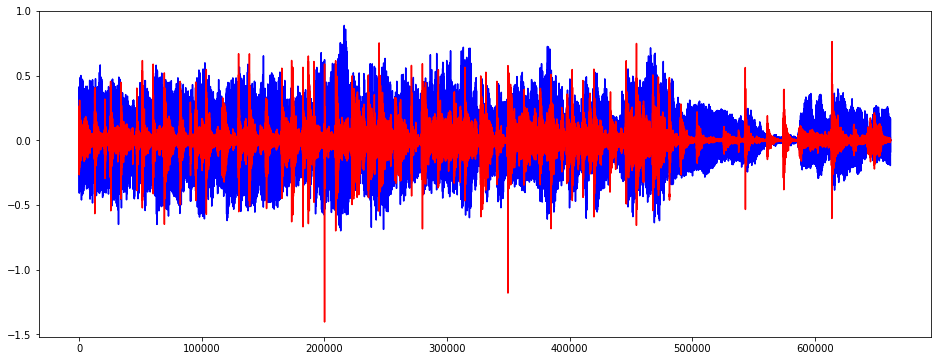
4.3.Harmonic and Percussive Components

楽曲データは様々な楽器音から構成されている。楽曲データを調波楽器音と打楽器音に分離する処理をHarmonic Percussive Source Separation: HPSSと呼ぶ．楽曲データを調波楽器音と打楽器音に分離してみる。（下記のページから転載）

#Harmonic and Percussive Components
y_harm, y_perc = librosa.effects.hpss(y)

plt.figure(figsize=(16, 6))
plt.plot(y_harm, color='b')
plt.plot(y_perc, color='r')
plt.show()

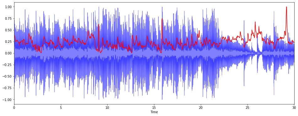
4.4.Spectral Centroid

音を周波数表現したとき、周波数の加重平均を計算して音の「重心」がどこかを知らせる指標。
たとえば、ブルース音楽は重心が中央部分に置かれているのに対し、メタル音楽は曲の最後の部分に重心が置かれる傾向がある。

spectral_centroids = librosa.feature.spectral_centroid(y, sr=sr)[0]

# Computing the time variable for visualization
frames = range(len(spectral_centroids))

# Converts frame counts to time (seconds)
t = librosa.frames_to_time(frames)

import sklearn
def normalize(x, axis=0):
  return sklearn.preprocessing.minmax_scale(x, axis=axis)

plt.figure(figsize=(16, 6))
librosa.display.waveplot(y, sr=sr, alpha=0.5, color='b')
plt.plot(t, normalize(spectral_centroids), color='r')
plt.show()

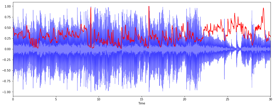
4.5.Spectral Rolloff

信号の形を測定する
総スペクトラルエネルギーの低い周波数（85％以下）にどのくらい集中しているかを見る。

#Spectral Rolloff
spectral_rolloff = librosa.feature.spectral_rolloff(y, sr=sr)[0]

plt.figure(figsize=(16, 6))
librosa.display.waveplot(y, sr=sr, alpha=0.5, color='b')
plt.plot(t, normalize(spectral_rolloff), color='r')
plt.show()

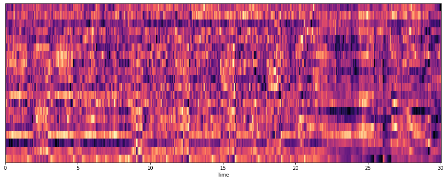
4.6.Mel-Frequency Cepstral Coefficients(MFCCs)

MFCCsは特徴の小さなセット（約10〜20）でスペクトラルフォー曲線の全体的な外観を省略して示す
人の聴覚構造を反映して、音声情報抽出

#Mel-Frequency Cepstral Coefficients (MFCCs)
mfccs = librosa.feature.mfcc(y, sr=sr)
mfccs = normalize(mfccs, axis=1)

print('mean: %.2f' % mfccs.mean())
print('var: %.2f' % mfccs.var())

plt.figure(figsize=(16, 6))
librosa.display.specshow(mfccs, sr=sr, x_axis='time')
plt.show()

mean: 0.50
var: 0.03

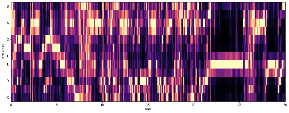
4.7.Chroma Frequencies

クロマの特徴は、音楽のエキサイティング強烈な表現である。
クロマは、人間の聴覚がオクターブ差がある周波数の2音を類似音であるかという音楽理論に基づいている。
すべてのスペクトルを、12個のBinで表現する。
12個のBinはオクターブで12個の異なる半音（Semitones = Chroma）を意味する。

#Chroma Frequencies

chromagram = librosa.feature.chroma_stft(y, sr=sr, hop_length=512)

plt.figure(figsize=(16, 6))
librosa.display.specshow(chromagram, x_axis='time', y_axis='chroma', hop_length=512)
plt.show()