ランダムフォレストで分類と回帰を行う

内容

ランダムフォレストを用いた分類と回帰モデルについてまとめます。
分類と回帰それぞれの結果の見方などを整理したいと思います。

実装内容

まずはライブラリをインポートします。

import pandas as pd
import numpy as np
import matplotlib.pyplot as plt
from sklearn.model_selection import train_test_split
from sklearn.metrics import mean_squared_error
from sklearn.metrics import mean_absolute_error
from sklearn.metrics import r2_score
from sklearn.metrics import accuracy_score

# ランダムフォレスト用のライブラリ
from sklearn.ensemble import RandomForestRegressor  #回帰モデル
from sklearn.ensemble import RandomForestClassifier  #分類モデル 

続いてデータを準備します。
データは前回の投稿と同じくIrisデータを用います。
ただし、irisデータは主に分類に用いるデータなので、
回帰モデルでは sepal length（cm) を目的変数としてモデルを構築します。

# データ読み込み
from sklearn.datasets import load_iris
iris = load_iris()
# データフレームを作成
data = pd.DataFrame(iris.data, columns=iris.feature_names)
# ターゲットデータを追加
data['target'] = iris.target

# 分類用データセット作成
x_cls = data.drop('target' , axis = 1)
y_cls = data['target']  

# 回帰用データセット作成
x_reg = data.drop(['target' , 'sepal length (cm)'] ,axis= 1)
y_reg = data['sepal length (cm)']

準備したデータセット
分類では目的変数をtarget、回帰では sepal length(cm) としてます。

続いて学習を行います。
まずは分類モデルで予測を行います。
ランダムフォレストは標準化が不要なので、そのまま学習を行います。

ランダムフォレスト　分類モデル

# データ分割（80%を学習用、20%をテスト用）
x_train, x_test, y_train, y_test = train_test_split(x_cls, y_cls, test_size=0.2, random_state=42)

# インスタンス化
model_clf = RandomForestClassifier(n_estimators=100, random_state=42)
# モデルの学習
model_clf.fit(x_train, y_train)

# 予測
y_pred = model_clf.predict(x_test)

# 評価（Accuracy）
accuracy = accuracy_score(y_test, y_pred)
print(f'Accuracy: {accuracy:.4f}')

結果

Accuracy: 1.0000

高精度で分類できることがわかります。
続いて特徴量の確認を行います。

# columnsを出力。スライスで最後の行以外（'target'以外）を得ています。
columns =  data.columns[: -1]

# DataFrame化
df_coef = pd.DataFrame(model_clf.feature_importances_ , index = columns , columns = ["feature"])

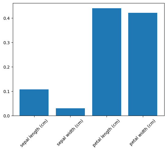
下記の結果が得られました。
この結果より分類にはpetal length (cm) と petal width (cm) が重要であることがわかります。

また合わせて特徴量の可視化も行います。

# 可視化
plt.bar(df_coef.index, df_coef["feature"])
# ラベルを45°にする
plt.xticks(rotation=45)
plt.show()

可視化により下記のグラフが得られました。

ここまでで回帰モデルが構築できました。
次に回帰モデルを構築します。

ランダムフォレスト　回帰モデル

回帰モデルも流れは同じですが、精度検証をする方法が異なります。

# データ分割（80%を学習用、20%をテスト用）
x_train, x_test, y_train, y_test = train_test_split(x_reg, y_reg, test_size=0.2, random_state=42)

# インスタンス化
model_reg = RandomForestRegressor(n_estimators=100, random_state=42)

# モデルの学習
model_reg.fit(x_train, y_train)

# モデルの予測
y_pred = model_reg.predict(x_test)

from sklearn.metrics import mean_absolute_error
from sklearn.metrics import mean_squared_error, r2_score

#MAE を計算
mae = mean_absolute_error(y_test, y_pred)
mse = mean_squared_error(y_test, y_pred)
rmse = np.sqrt(mse)
r2 = r2_score(y_test, y_pred)

# 精度を出力
print(f'Mean Squared Error: {mse:.4f}')
print(f'Root Mean Squared Error: {rmse:.4f}')
print(f'R² Score: {r2:.4f}')
print(f'Mean Absolute Error: {mae:.4f}')

出力結果は下記になります。

Mean Squared Error: 0.0974
Root Mean Squared Error: 0.3121
R² Score: 0.8588
Mean Absolute Error: 0.2571

こちらは決定係数$R^2$が0.8588となり分類時よりも精度が低い結果となりました。

ハイパーパラメータを変更していないので、改善の余地はあるかもしれません。

最後に特徴量の可視化を行います。

# columnsを出力。説明変数から取り出し
columns =  x_reg.columns

# DataFrame化
df_coef = pd.DataFrame(model_reg.feature_importances_ , index = columns , columns = ["feature"])

# 可視化
plt.bar(df_coef.index, df_coef["feature"])
# ラベルを45°にする
plt.xticks(rotation=45)
plt.show()

結果よりsepal length（がく片の長さ）はpetal length（花びらの長さ）が重要な要素であることがわかりました。
今後ハイパーパラメータの最適化の方法をまとめたいと思います。