はじめに
Rを学びたいStep13です。今回は単回帰分析について学びます
単回帰分析とは
単回帰分析(Simple Linear Regression)は、1つの独立変数(説明変数)を使って、1つの従属変数(目的変数)を予測したり、変数間の関係を理解するための統計手法です。
単回帰分析の指揮
単回帰分析では、データ間の関係を一次関数(直線) で表します。
この直線は次の式で表されます:
y = \beta_0 + \beta_1 x + \varepsilon
\begin{align*}
1. \quad y &: \text{従属変数(目的変数)} \\
&\bullet \text{予測したい対象の値。} \\
&\bullet \text{例: 売上、テストの点数、体重の減少など。} \\
\\
2. \quad x &: \text{独立変数(説明変数)} \\
&\bullet \text{従属変数に影響を与えると考えられる要因。} \\
&\bullet \text{例: 広告費、勉強時間、運動時間など。} \\
\\
3. \quad \beta_0 &: \text{切片(Intercept)} \\
&\bullet x = 0 \text{ のときの } y \text{ の値。} \\
&\bullet \text{例: 広告費を全く使わない場合の売上、勉強を全くしない場合の点数。} \\
\\
4. \quad \beta_1 &: \text{傾き(Slope)} \\
&\bullet x \text{ が1単位増えると } y \text{ がどれだけ増加または減少するかを示す。} \\
&\bullet \text{正の値であれば } x \text{ の増加に伴って } y \text{ が増加し、負の値であれば減少する。} \\
\\
5. \quad \varepsilon &: \text{誤差項(Error Term)} \\
&\bullet \text{実際の値(観測値)と、モデルが予測した値(回帰直線上の値)とのズレ。} \\
&\bullet \text{例: データに含まれる測定誤差やモデル化されていない他の要因の影響。}
\end{align*}
単回帰分析の例
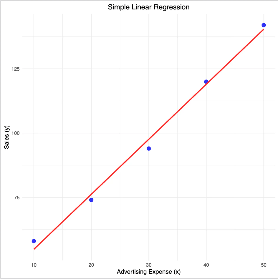
今回は広告費と売り上げに関する単回帰分析を実施していきます。

1. 平均値を求める
広告費、売り上げの平均を算出する
\bar{x} = \frac{10 + 20 + 30 + 40 + 50}{5} = \frac{150}{5} = 30
\bar{y} = \frac{58 + 74 + 94 + 120 + 142}{5} = \frac{488}{5} = 97.6
2. 偏差を計算
\begin{array}{|c|c|c|c|}
\hline
x_i & x_i - \bar{x} & y_i & y_i - \bar{y} \\
\hline
10 & 10 - 30 = -20 & 58 & 58 - 97.6 = -39.6 \\
20 & 20 - 30 = -10 & 74 & 74 - 97.6 = -23.6 \\
30 & 30 - 30 = 0 & 94 & 94 - 97.6 = -3.6 \\
40 & 40 - 30 = 10 & 120 & 120 - 97.6 = 22.4 \\
50 & 50 - 30 = 20 & 142 & 142 - 97.6 = 44.4 \\
\hline
\end{array}
3. 偏差の積と偏差の2乗を計算
\begin{array}{|c|c|c|c|}
\hline
x_i - \bar{x} & y_i - \bar{y} & (x_i - \bar{x})(y_i - \bar{y}) & (x_i - \bar{x})^2 \\
\hline
-20 & -39.6 & (-20) \times (-39.6) = 792.0 & (-20)^2 = 400 \\
-10 & -23.6 & (-10) \times (-23.6) = 236.0 & (-10)^2 = 100 \\
0   & -3.6  & 0 \times (-3.6) = 0.0        & 0^2 = 0       \\
10  & 22.4  & 10 \times 22.4 = 224.0       & 10^2 = 100    \\
20  & 44.4  & 20 \times 44.4 = 888.0       & 20^2 = 400    \\
\hline
\end{array}
4. 偏差の積と偏差の2乗の総和を計算
\begin{aligned}
\sum (x_i - \bar{x})(y_i - \bar{y}) &= 792.0 + 236.0 + 0.0 + 224.0 + 888.0 \\
&= 2140.0 \\
\\
\sum (x_i - \bar{x})^2 &= 400 + 100 + 0 + 100 + 400 \\
&= 1000
\end{aligned}
5. 傾きの計算
傾きの公式:

\beta_1 = \frac{\sum (x_i - \bar{x})(y_i - \bar{y})}{\sum (x_i - \bar{x})^2}
\beta_1 = \frac{2140.0}{1000} = 2.14
6. 切片 を計算
切片の公式:

\beta_0 = \bar{y} - \beta_1 \bar{x}
数値を代入:

\beta_0 = 94 - 2.14 \times 30 = 97.6 - 64.2 = 29.8
ソースコード
前段階の説明が長くなってしまいましたが、Rで実装していこうと思います。
# 必要なライブラリ
library(ggplot2)
library(extrafont)  # フォント管理ライブラリ

# 日本語対応フォントをインストール(必要に応じて一度だけ実行)
# font_import(prompt = FALSE)

# 日本語フォントの指定
jp_font <- "Hiragino Sans"  # Macの場合 (ヒラギノ)
# jp_font <- "MS Gothic"  # Windowsの場合

# データの作成
data <- data.frame(
  x = c(10, 20, 30, 40, 50),  # 広告費
  y = c(58, 74, 94, 120, 142) # 売上
)

# 単回帰分析の計算
mean_x <- mean(data$x)  # xの平均
mean_y <- mean(data$y)  # yの平均

# 傾きと切片の計算
sum_xy <- sum((data$x - mean_x) * (data$y - mean_y))
sum_x2 <- sum((data$x - mean_x)^2)
beta_1 <- sum_xy / sum_x2  # 傾き
beta_0 <- mean_y - beta_1 * mean_x  # 切片

# 回帰直線の方程式
data$y_pred <- beta_0 + beta_1 * data$x

# プロットの作成
ggplot(data, aes(x = x, y = y)) +
  geom_point(color = "blue", size = 3, alpha = 0.8) +  # 元のデータ点
  geom_line(aes(y = y_pred), color = "red", size = 1) + # 回帰直線
  labs(
    title = "単回帰分析のプロット",
    x = "広告費 (x)",
    y = "売上 (y)"
  ) +
  theme_minimal(base_family = jp_font) +  # 日本語フォントを指定
  theme(plot.title = element_text(hjust = 0.5))  # タイトル中央寄せ
最後に
単回帰分析の説明でした!コードにすると意外とシンプルです!!