Learning curve について
Learning Curve(学習曲線)については、scikit-learnのValidation curves: plotting scores to evaluate modelsやPlotting Learning Curvesに書かれています。
ざっくり説明すると、構築した学習モデルが過学習の傾向が強くなっていないかを調べるということ。
トレーニングデータを使って構築した学習モデルが、テストデータを入力した時に、トレーニングデータに大きく依存しているものになると、テストデータに対しては、うまく分類する事ができなくなってしまいます。そのトレーニングデータへの依存度の傾向を知る為に、学習曲線を使います!
今回は、このLearning CurveをPython3でやってみます。
AnacondaのJupyter Notebookを用いて行います。
ライブラリのインストール
sklearnのversion確認
import sklearn
print('The scikit-learn version is {}.'.format(sklearn.__version__))
The scikit-learn version is 0.19.1.
import pandas as pd
import numpy as np
import matplotlib.pyplot as plt
from sklearn.svm import SVC
from sklearn.model_selection import train_test_split
from sklearn.cross_validation import ShuffleSplit
from sklearn.model_selection import GridSearchCV
from sklearn.learning_curve import learning_curve
Pythonでsklearnのgrid searchが使えないときの対処方法
この記事とか参考にしました。
versionでインストールのコードの書き方が少し異なります。
plot_learning_curve
scikit-learnのplot_learning_curve()を拝借してきます。
def plot_learning_curve(estimator, title, X, y, ylim=None, cv=5, n_jobs=4, train_sizes=np.linspace(0.1, 1.0, 10)):
    plt.figure()
    plt.title(title)
    if ylim is not None:
        plt.ylim(*ylim)
    plt.xlabel('Number of training samples', fontsize=14)
    plt.ylabel('Score', fontsize=14)
    plt.tick_params(labelsize=14)
    train_sizes, train_scores, test_scores = learning_curve(
        estimator, X, y, cv=cv, n_jobs=n_jobs, train_sizes=train_sizes)
    train_scores_mean = np.mean(train_scores, axis=1)
    train_scores_std = np.std(train_scores, axis=1)
    test_scores_mean = np.mean(test_scores, axis=1)
    test_scores_std = np.std(test_scores, axis=1)
    plt.grid()

    plt.fill_between(train_sizes, train_scores_mean - train_scores_std,
                     train_scores_mean + train_scores_std, alpha=0.1,
                     color="r")
    plt.fill_between(train_sizes, test_scores_mean - test_scores_std,
                     test_scores_mean + test_scores_std, alpha=0.1, color="g")
    plt.plot(train_sizes, train_scores_mean, 'o-', color="r",
             label="Training score")
    plt.plot(train_sizes, test_scores_mean, 'o-', color="g",
             label="Cross-validation score")

    plt.legend(loc="best")
    return plt
データの読み込みからモデルの作成まで
# Load the dataset
df = pd.read_csv('sample.csv')
# 正解ラベルを除く特徴量をxに
# Classの部分に、csvデータのクラスを表す名前をいれてください
X = df.drop(['Class'], axis=1)
# 正解ラベルをyに
y = df['Class']
# Split into training and test set
X_train, X_test, y_train, y_test = train_test_split(X, y, test_size=0.2, random_state=0)
# Choose estimator
estimator = SVC(kernel='linear')
# Choose cross-validation iterator
cv = ShuffleSplit(X_train.shape[0], n_iter=10, test_size=0.2, random_state=42)
# Tune the hyperparameters
gammas = np.logspace(-6, -1, 10)
classifier = GridSearchCV(estimator=estimator, cv=cv, param_grid=dict(gamma=gammas))
classifier.fit(X_train, y_train)
実行結果
GridSearchCV(cv=ShuffleSplit(440, n_iter=10, test_size=0.2, random_state=42),
       error_score='raise',
       estimator=SVC(C=1.0, cache_size=200, class_weight=None, coef0=0.0,
  decision_function_shape='ovr', degree=3, gamma='auto', kernel='linear',
  max_iter=-1, probability=False, random_state=None, shrinking=True,
  tol=0.001, verbose=False),
       fit_params=None, iid=True, n_jobs=1,
       param_grid={'gamma': array([1.00000e-06, 3.59381e-06, 1.29155e-05, 4.64159e-05, 1.66810e-04,
       5.99484e-04, 2.15443e-03, 7.74264e-03, 2.78256e-02, 1.00000e-01])},
       pre_dispatch='2*n_jobs', refit=True, return_train_score='warn',
       scoring=None, verbose=0)
色々チューニングしています
学習曲線のプロット
# Debug algorithm with learning curve
title = 'Learning Curves (SVM, linear kernel, $\gamma=%.6f$)' %classifier.best_estimator_.gamma
estimator = SVC(kernel='linear', gamma=classifier.best_estimator_.gamma)
plot_learning_curve(estimator, title, X_train, y_train, cv=cv)
plt.show()
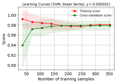
プロットできました。
うっすら色がついているのは、交差検証しているからです。
scikit-learn を用いた交差検証(Cross-validation)とハイパーパラメータのチューニング(grid search)とかの記事に詳しくあるので、ここでは説明飛ばします。
データセットが200を超えたくらいから98%の精度を維持しているのが嬉しいですね。
このデータセットは自分が研究で使用しているものですが、少し特徴量を減らして学習曲線をプロットしてみます。
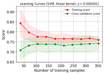
少しグラフの雰囲気が変わりましたね。
そのモデル、過学習してるの?未学習なの?と困ったら
この記事に、ここらへんの説明がされています。
さっき取り除いた特徴量は、良いモデルを作成する為に結構貢献している特徴量でした。
学習曲線を使うことで、モデルのoverfittingやunderfittingを確認できるので、ただモデルの精度を語るより、説得力のある話ができるのが強みだと思います。