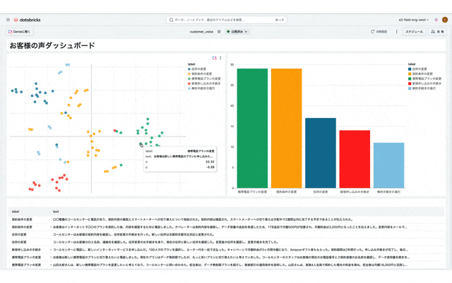
お客様の声(Voice of Customer)をグループ化して可視化したダッシュボード
目次
はじめに
"If you don’t listen to your customers, someone else will."
とビジネスで良く言われるかと思います。自社が顧客の声を聞いて活用しなければ、競合が製品/サービスを改善して顧客を取っていきます。顧客を取られないように皆様の組織では顧客の声をどのように収集し、活用していますでしょうか。
組織によって向き合い方は千差万別だと思いますが、顧客フィードバックは、収益向上と競争力強化に不可欠です。A Research Paper on the Effects of Customer Feedback on Businessという研究によると、満足した顧客はリピート購入を通じてブランドロイヤルティを高め、5~6人に良い体験を共有します。特に、「完全に満足した顧客」は「やや満足した顧客」に比べ、収益貢献度が2.6倍高いことが示されています。さらに、顧客維持率を5%向上させるだけで利益が最大75%増加する可能性があり、顧客の声に応える重要性が明らかです。
しかし、SNS、メール、アンケートなど顧客の声が多様なチャネルに分散する現在、継続的かつ効率的なフィードバック収集は多くの企業にとって課題になっているかと思います。データ統合やチャネル間の調整が難しく、顧客体験の全体像を把握できない企業が多いのが現状です。
本記事ではデータブリックスを活用することで、大量の顧客フィードバックを効率的に分析・可視化する方法を書いていきます。
今後も記事執筆を継続するモチベーションに繋がりますので「いいね」や記事の保存、SNSで共有いただけると嬉しいです。 宜しくお願いいたします!
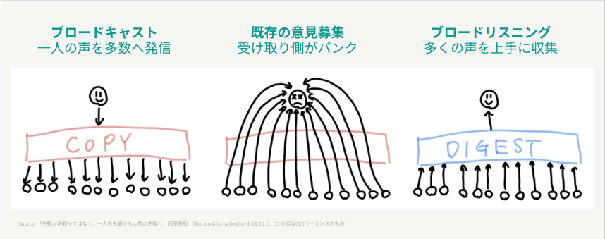
ブロードリスニングとは何か
ブロードリスニングという言葉を知ってますか?
説明は多くの記事でなされているので簡単にさせていただきますが、端的にいうと
「広範囲に人の意見を収集し、収集した意見をAIで分析・可視化する手法」
かと思います。為政者が有権者の声を一つずつ聞くのではなく、経営者が顧客の声を一つずつ聞くのではなく、大枠の傾向としてどんなことを言っているのかを把握する際に使われる技術です。
↓良く見る図
2024年の都知事選で安野貴博さんというAIエンジニアの方が都議会の議事録要約やSNSの分析に用いて話題になりました。
GovTech東京アドバイザーとして、安野がこれから「東京の未来」のために活用していく「ブロードリスニング」📊
— 安野たかひろスタッフ@チームみらい【公式】 (@annotakahiro24) November 22, 2024
どんな手法なのか?どのように民意をAIで反映させていくのか?
10分でわかるYouTubeライブのまとめ動画を公開しました!
ぜひご覧ください🎥https://t.co/qtMCbQGxZU pic.twitter.com/WjOzCfMlQB
AI Objective Instituteが出している「Talk To The City」というフレームワークを日本語で対応可能なように改変して使われていたようです。
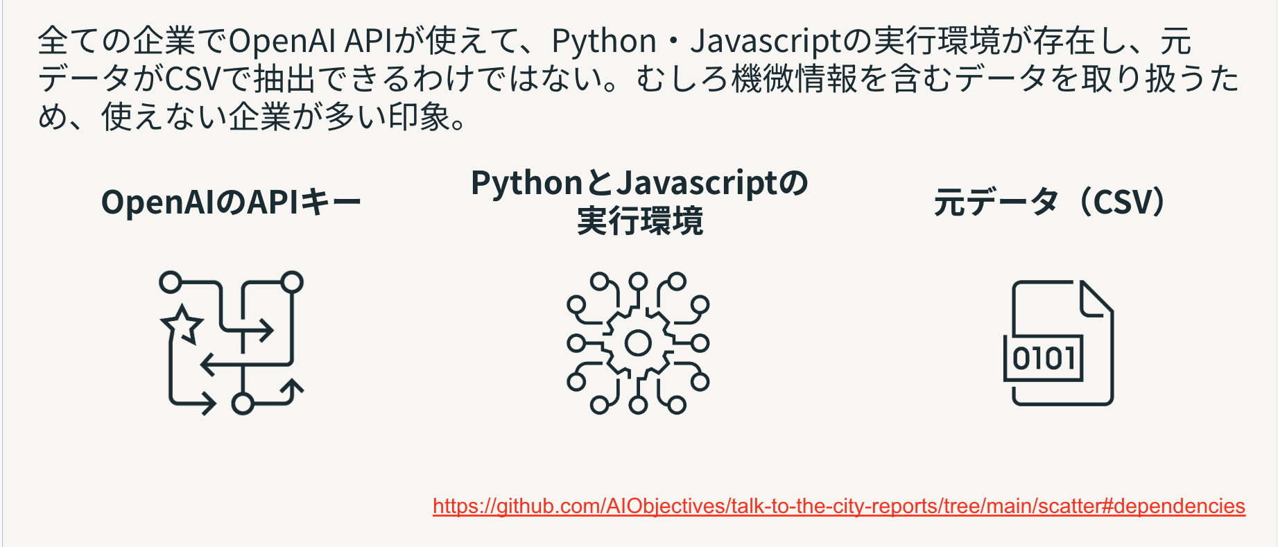
自分も作ってみましたが、下記(公式の要件)を満たせば簡単にレポートが作成できます。
- OpenAIのAPIアクセス
- Python並びにJavascript実行環境
- ダウンロードされたCSV
一方で一般的な企業に勤めている方々が利用しようと思うと、下記を含めて様々な課題に直面する場合があるかと思います。
- OpenAIのAPIが利用できない
- PythonとJavascriptの環境が存在しない、また構築にも時間を要する
- レポートを開発・メンテナンスするスキルを持った人材がいない
- 機微情報を含むデータをダウンロード/アップロードできない
以下では上記の課題を解消しながら、クイックにお客様の声を分析できるようにチュートリアルを実施できればと思います。次の章で詳細なステップを見ていきます。
データブリックスを用いたお客様の声分析
Talk To The City のGitHubを見ると処理の内容を把握できます。その中でも main.py を見ると大枠のStepは下記9ステップでテキスト整形後にエンべディング、クラスタリング、ラベリング、可視化を実施していることがわかります。
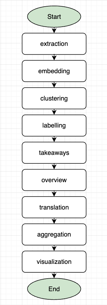
今回は日本語のテキストを用いるため翻訳などのステップが不要なので削除して、必要な箇所のみをデータブリックスの実装に変換しながら進めていきます。
データ作成
今回はコールセンター業務において、お客様とオペレータの会話がテキスト化されていると想定して、Databricks上で利用できる Llama4 を用いて独自のデータセットを100行作っていきます。
CATALOG = "kohei_arai"
SCHEMA = "demo"
TABLE = "calls_log"

# Create widgets for CATALOG and SCHEMA
dbutils.widgets.text("CATALOG", CATALOG)
dbutils.widgets.text("SCHEMA", SCHEMA)
dbutils.widgets.text("TABLE", TABLE)

# Get the widget values
catalog = dbutils.widgets.get("CATALOG")
schema = dbutils.widgets.get("SCHEMA")
table = dbutils.widgets.get("TABLE")
from pyspark.sql.functions import col, lit, rand, floor, when

# Create a DataFrame with 100 records
df = spark.range(100).withColumnRenamed("id", "call_id")

# Define the categories
categories = ["契約内容の確認・変更", "料金や請求に関する確認", "解約や休止の申請・手続き", "個人情報の変更(住所・連絡先など)", "新規申し込みやサービス追加の依頼"]

# Add the category column with random values from the categories list
df = df.withColumn(
    "category",
    when(floor(rand() * len(categories)) == 0, lit(categories[0]))
    .when(floor(rand() * len(categories)) == 1, lit(categories[1]))
    .when(floor(rand() * len(categories)) == 2, lit(categories[2]))
    .when(floor(rand() * len(categories)) == 3, lit(categories[3]))
    .otherwise(lit(categories[4]))
)

# Display the DataFrame
df.createOrReplaceTempView("calls_id")
display(df)
データブリックスだとai_queryという関数が用意されており、SQL内でAIモデルにクエリを投げることができ、下記のようにデータ作成にも使えます。AIモデルをスクラッチで書かなくても、10行程度のSQLを書くことでAIにアクセスできて便利です。
# Create the SQL query using the widget values
query = f"""
CREATE OR REPLACE TABLE `{catalog}`.`{schema}`.`{table}`
SELECT
  call_id,
  ai_query(
    "databricks-llama-4-maverick",
    "貴方はコールセンターの会話に精通するプロフェッショナルです。カテゴリを加味して、コールセンターのやりとりを想定して会話を作成してください。call_idが違う場合は違う会話を想定してください。Call ID:" || call_id || "Category:" || category
  ) AS content
FROM calls_id
"""

# Run the SQL query
spark.sql(query)
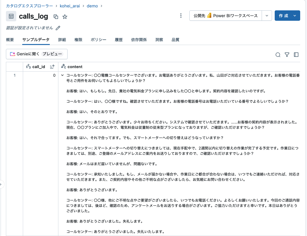
クエリ終了後にカタログでテーブルを検索してみると通話履歴データが作成・格納されていることがわかります。内容としても問題ないことが確認できるので次のステップに進みます。
テキストサマリ
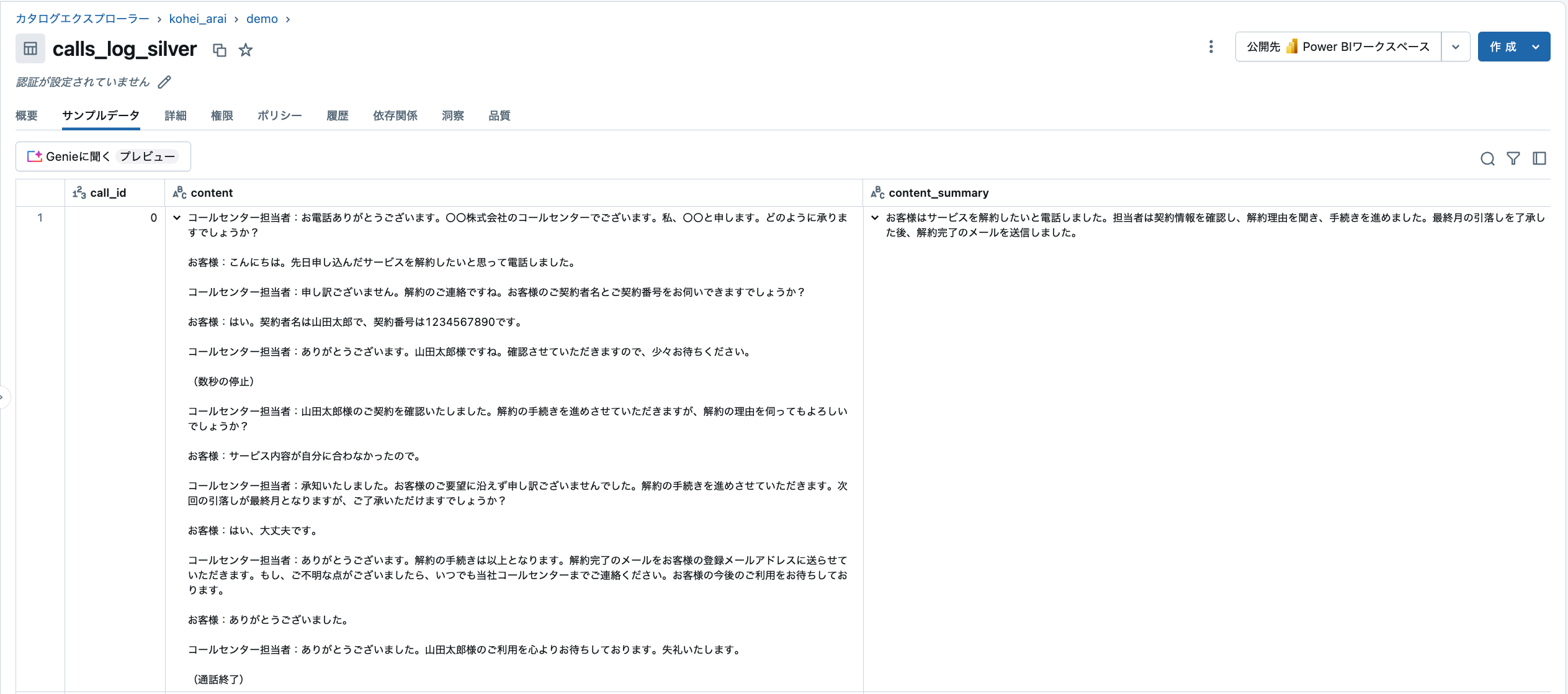
前のステップで作成した通話ログは「こんにちは」など会話において特段意味を持たないフレーズが含まれているため、必要な情報のみを抽出します。前述のai_query()関数を使用して今回はLlama3.3 70Bにクエリを投げて、サマリ列を追加したテーブルを作成します。
CREATE OR REPLACE TABLE calls_log_silver AS
SELECT
  call_id,
  content,
  ai_query(
    "databricks-meta-llama-3-3-70b-instruct",
    "貴方は日本語を端的かつ分かりやすく要約するプロフェッショナルです。与えられた文章を日本語で100文字程度に要約してください。時制は過去形で返してください。結果からは人名やメールアドレス・電話番号といった個人情報はのぞいてください"
    || `content`
  ) AS content_summary
FROM
  calls_log;
こちらも結果を見てみるとちゃんと要約が作られていることがわかります。
元のテキスト
コールセンター: 〇〇電機コールセンターでございます。お電話ありがとうございます。私、山田がご対応させていただきます。お客様の電話番号とご用件をお伺いしてもよろしいでしょうか?
お客様: はい、もしもし。先日、貴社の電気料金プランに申し込みをした〇〇と申します。契約内容を確認したいのですが。
コールセンター: はい、〇〇様ですね。確認させていただきます。お客様の電話番号はお電話いただいている番号でよろしいでしょうか?
お客様: はい、そのとおりです。
コールセンター: ありがとうございます。少々お待ちください。システムで確認させていただきます。……お客様の契約内容が表示されました。現在、〇〇プランにご加入中で、電気料金は従量制の従来型プランになっておりますが、ご確認いただけますでしょうか?
お客様: はい、それで合ってます。でも、スマートメーターへの切り替えはどうなっていますか?
コールセンター: スマートメーターへの切り替えにつきましては、現在手配中で、2週間以内に切り替えの作業が完了する予定です。作業日につきましては、別途、ご登録のメールアドレスにご案内をお送りしておりますので、ご確認いただけますでしょうか?
お客様: メールはまだ届いていませんが、問題ないです。
コールセンター: 承知いたしました。もし、メールが届かない場合や、作業日にご都合が合わない場合は、いつでもご連絡いただければ、対応させていただきます。また、ご契約内容やその他ご不明な点がございましたら、お気軽にお問い合わせください。
お客様: ありがとうございます。
コールセンター: 〇〇様、他にご不明な点やご要望がございましたら、いつでもお電話ください。よろしくお願いいたします。今回のご通話内容につきましては、後ほど、確認のため、アンケートメールをお送りする場合がございます。ご協力いただけますと幸いです。本日はありがとうございました。
お客様: ありがとうございました。失礼します。
コールセンター: ありがとうございました。失礼いたします。
サマリ
〇〇電機のコールセンターに電話があり、契約内容の確認とスマートメーターへの切り替えについて相談された。契約内容は確認され、スマートメーターへの切り替えは手配中で2週間以内に完了する予定であることが伝えられた。
このステップの精度が悪い場合は、要約で使っているモデルを変える必要がありますが、
綺麗な要約になっていることが確認できましたので次のステップに進みます。
ベクトル化
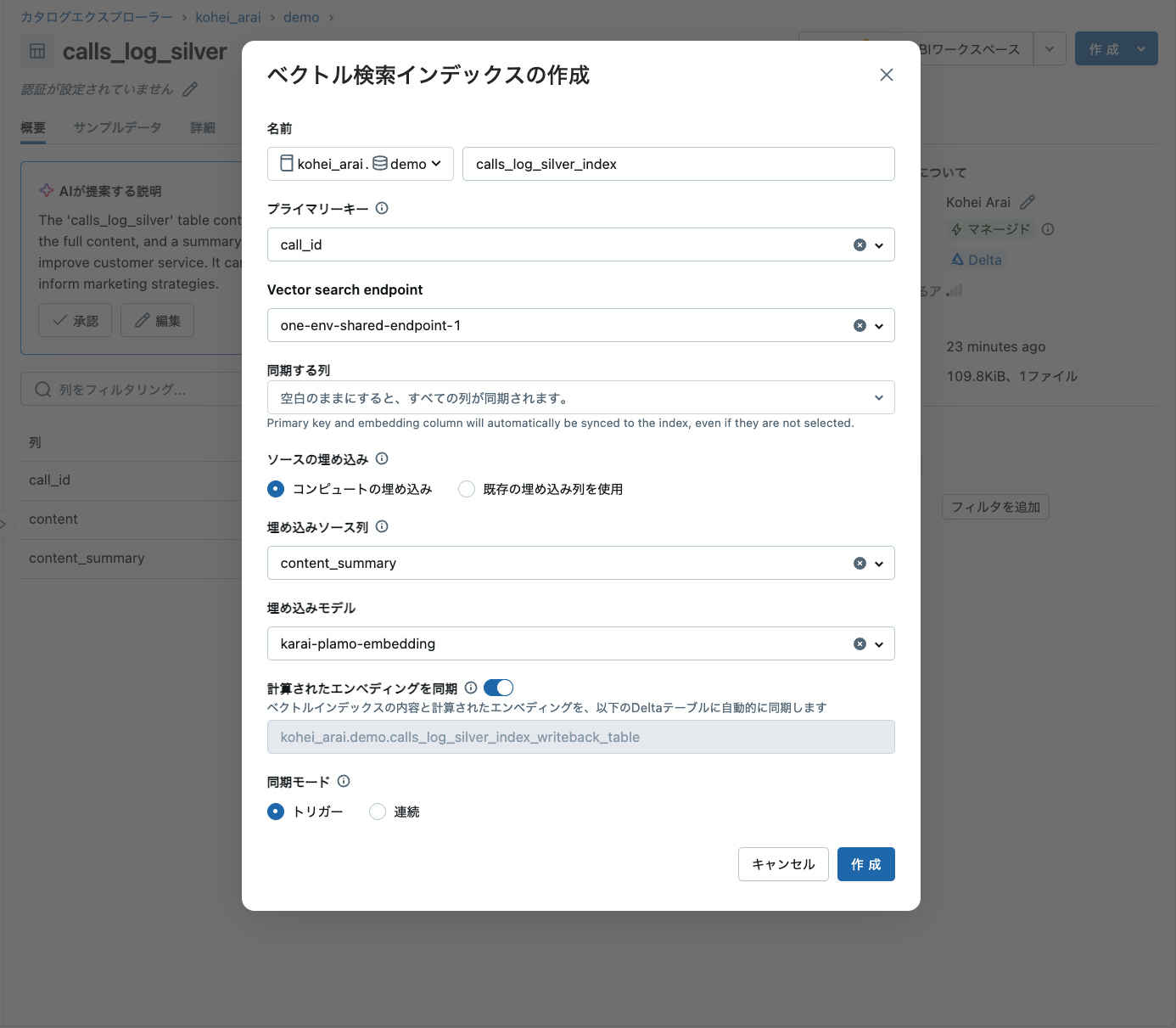
次にクラスタリングを実施するためにサマリされたテキストをベクトル化していきます。DatabricksにおいてはVector Searchを使っていきます。ChangeDataFeedを有効化していないと、Vector Searchがソーステーブルとして使えないので下記クエリを実行して有効化しておきます。
ALTER TABLE `kohei_arai`.`demo`.`calls_log_silver` SET TBLPROPERTIES (delta.enableChangeDataFeed = true);
テーブルのページから下記のように設定します。埋め込みモデルをお好きなモデルを使っていただければと思いますが、今回はPLaMoを使用しております。Databricksでカスタムモデルをデプロイする方法はドキュメントをご参照ください。
ここで忘れてはいけない点として「計算されたエンべディングを同期」をオンにしてください。計算されるベクトルを使用してこの後のステップでクラスタリングを行いますが、デフォルトだとテーブルが生成されないため、こちらのオプションをオンにしてベクトル列を含んだテーブルを生成するようにします。
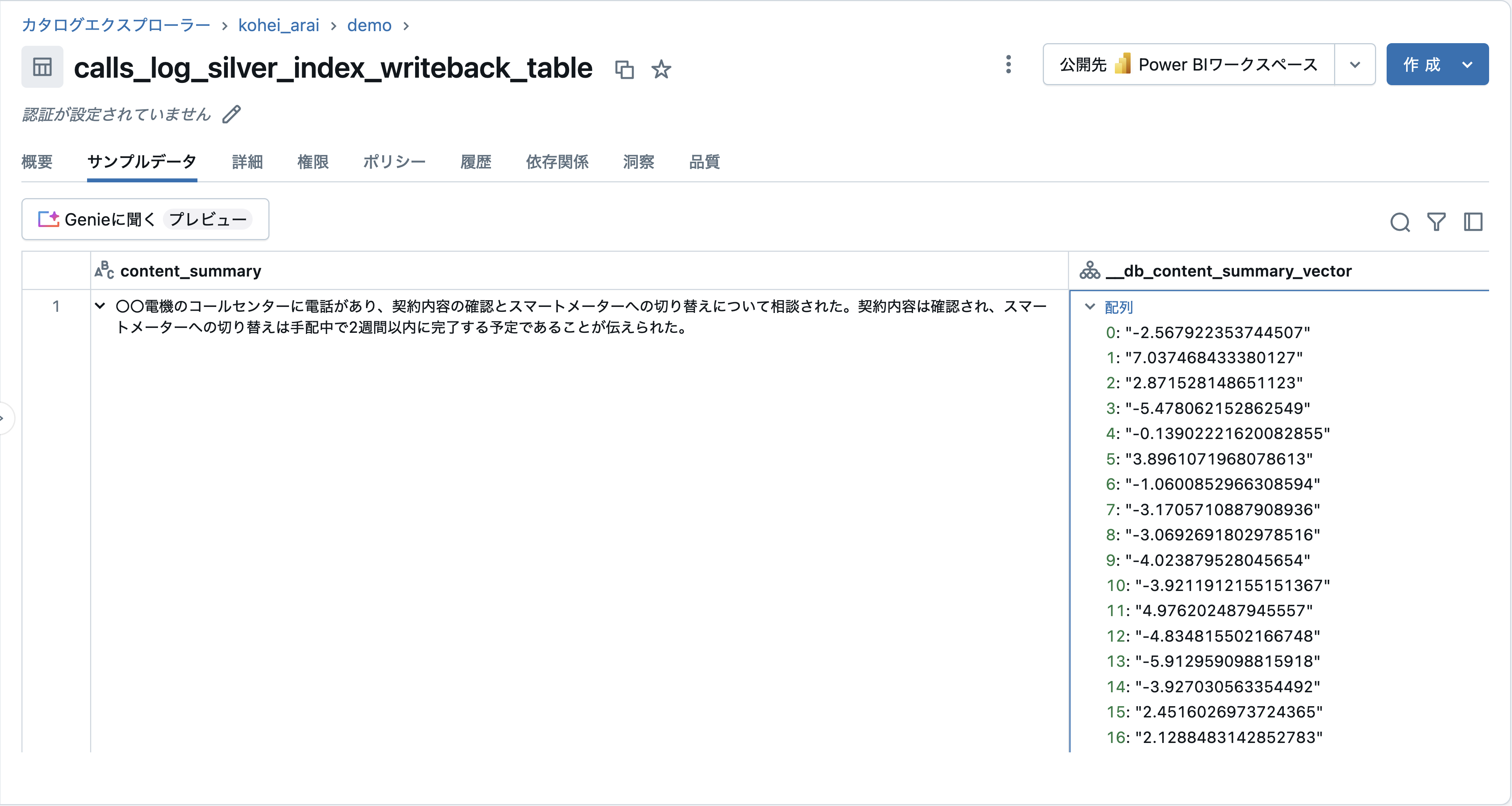
作成に2-3分ほどかかりますが、結果を見てみるとwriteback_tableにサマリが2048次元のベクトル列が追加されていることがわかります。このベクトルを使用してこの後のステップではクラスタリングを行なっていきます。
クラスタリング
次に作成したベクトルを使ってグループを作成します。まずは必要なパッケージをインストールします。
!pip install umap-learn numpy hdbscan bertopic langchain databricks-sdk[openai]
本家のコードをデータブリックスで実行できるように変更しており、下記を実行します。
こちらのスクリプトを実行すると2048次元のベクトルを用いてスペクトルクラスタリングの手法でクラスタを作成します。
from pyspark.sql import functions as F
from pyspark.ml.feature import VectorAssembler
from sklearn.cluster import SpectralClustering
from sklearn.metrics import silhouette_score
import numpy as np
from pyspark.sql.types import IntegerType
import pandas as pd
def prepare_data(spark_df, vector_col="__db_content_summary_vector"):
"""
Convert Spark DataFrame to numpy array for sklearn
"""
# Convert to pandas first (more efficient for spectral clustering)
pandas_df = spark_df.toPandas()
# Convert string representation of array to numpy array if needed
if isinstance(pandas_df[vector_col][0], str):
vectors = np.array([eval(v) for v in pandas_df[vector_col]])
else:
vectors = np.array(pandas_df[vector_col].tolist())
return vectors, pandas_df
def find_optimal_clusters(X, max_clusters=10):
"""
Find optimal number of clusters using silhouette score
"""
silhouette_scores = []
for n_clusters in range(2, max_clusters + 1):
print(f"Testing {n_clusters} clusters...")
# Initialize and fit Spectral Clustering
spectral = SpectralClustering(
n_clusters=n_clusters,
assign_labels='discretize',
random_state=42,
affinity='nearest_neighbors' # Using KNN for sparse affinity matrix
)
cluster_labels = spectral.fit_predict(X)
# Calculate silhouette score
score = silhouette_score(X, cluster_labels)
silhouette_scores.append(score)
print(f"Silhouette score for {n_clusters} clusters: {score:.3f}")
optimal_clusters = np.argmax(silhouette_scores) + 2
return optimal_clusters
def perform_spectral_clustering(X, n_clusters):
"""
Perform spectral clustering with optimal parameters
"""
spectral = SpectralClustering(
n_clusters=n_clusters,
assign_labels='discretize',
random_state=24,
affinity='nearest_neighbors',
n_neighbors=10 # Adjust based on your data
)
return spectral.fit_predict(X)
def create_spark_df_with_clusters(spark, original_df, cluster_labels):
"""
Create a new Spark DataFrame with cluster assignments
"""
# Convert cluster labels to Spark DataFrame
cluster_pd = pd.DataFrame(cluster_labels, columns=['cluster_id'])
cluster_spark = spark.createDataFrame(cluster_pd)
# Add row index to both DataFrames
original_with_index = original_df.withColumn("row_idx", F.monotonically_increasing_id())
cluster_with_index = cluster_spark.withColumn("row_idx", F.monotonically_increasing_id())
# Join the DataFrames
return original_with_index.join(
cluster_with_index,
on="row_idx"
).drop("row_idx")
# Main clustering pipeline
def spectral_clustering_pipeline(spark_df, max_clusters=10, n_clusters=None):
"""
Main pipeline for spectral clustering
"""
print("Preparing data...")
X, pandas_df = prepare_data(spark_df)
if n_clusters is None:
print("Finding optimal number of clusters...")
# n_clusters = find_optimal_clusters(X, max_clusters)
n_clusters = max_clusters
print(f"Optimal number of clusters: {n_clusters}")
print(f"Performing spectral clustering with {n_clusters} clusters...")
cluster_labels = perform_spectral_clustering(X, n_clusters)
# Create final DataFrame with cluster assignments
final_df = create_spark_df_with_clusters(spark, spark_df, cluster_labels)
# Show cluster distribution
print("\nCluster distribution:")
final_df.groupBy("cluster_id").count().orderBy("cluster_id").show()
return final_df
# Run the pipeline
clustered_df = spectral_clustering_pipeline(
df,
max_clusters=5 # Adjust based on your needs
)
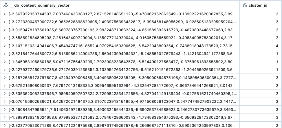
display(clustered_df)
実行結果として下図のように、それぞれのベクトルがクラスタに分類された結果が得られます。
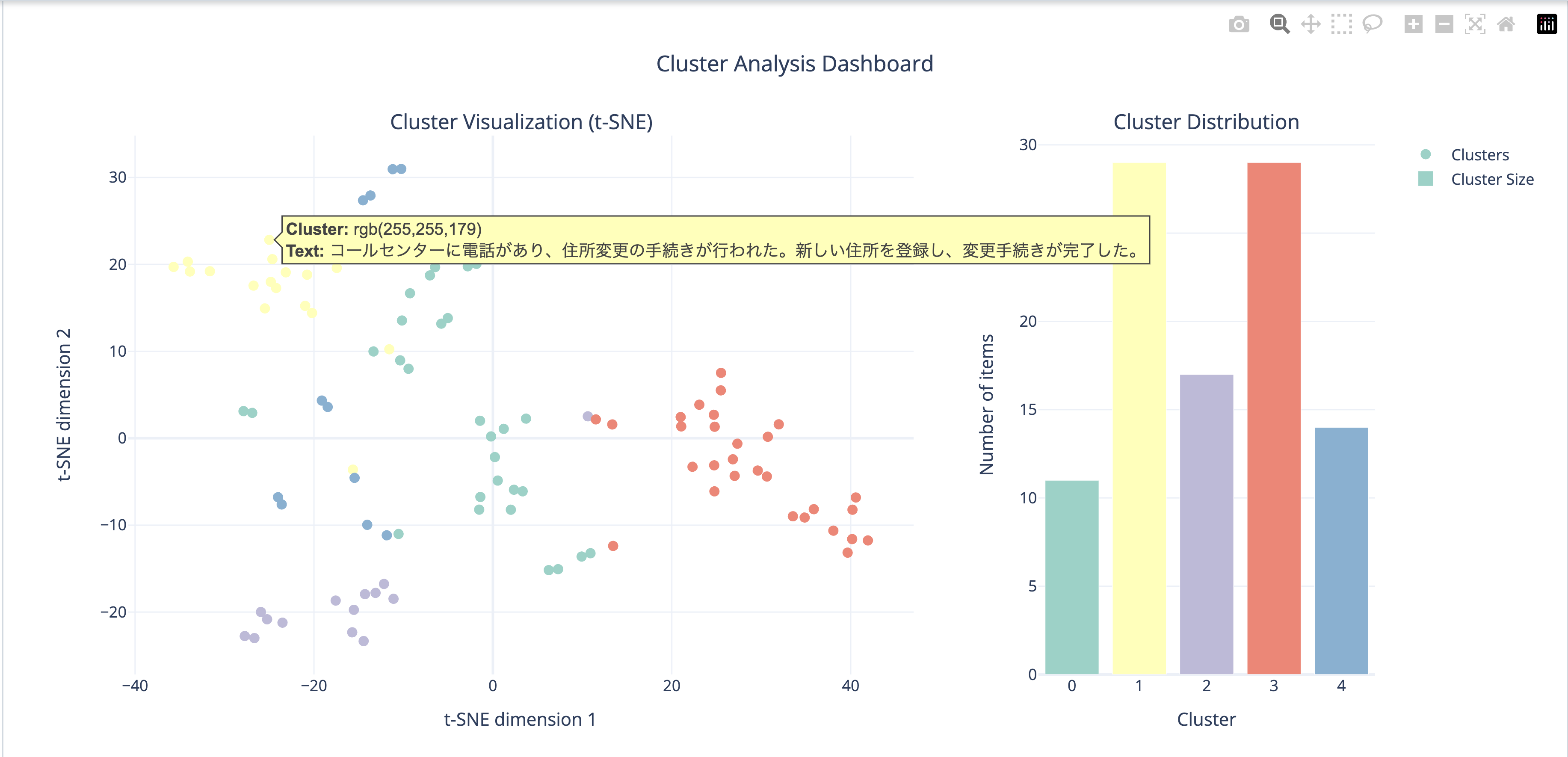
可視化を行なっていきますが2048次元のベクトルだと描画ができないので、t-SNEを用いて描画用に2次元のベクトルに圧縮します。
import numpy as np
import pandas as pd
from sklearn.manifold import TSNE
import plotly.express as px
import plotly.graph_objects as go
from plotly.subplots import make_subplots

# Convert embeddings to numpy array
vectors = np.array(clustered_df.select('__db_content_summary_vector').toPandas()['__db_content_summary_vector'].tolist())
clusters = np.array(clustered_df.select('cluster_id').toPandas()['cluster_id'].tolist())
texts = clustered_df.select('content_summary').toPandas()['content_summary'].tolist()

# Perform t-SNE
print("Performing t-SNE dimensionality reduction...")
tsne = TSNE(n_components=2, random_state=42, perplexity=5)
embeddings_2d = tsne.fit_transform(vectors)

# Create DataFrame for plotting
plot_df = pd.DataFrame({
    'x': embeddings_2d[:, 0],
    'y': embeddings_2d[:, 1],
    'cluster': clusters.astype(str),  # Convert to string for better legends
    'text': texts
})

# Map cluster IDs to colors
unique_clusters = plot_df['cluster'].unique()
color_map = {cluster: px.colors.qualitative.Set3[i % len(px.colors.qualitative.Set3)] for i, cluster in enumerate(unique_clusters)}
plot_df['color'] = plot_df['cluster'].map(color_map)

# Create subplots: main scatter plot and cluster distribution
fig = make_subplots(
    rows=1, cols=2,
    column_widths=[0.7, 0.3],
    specs=[[{"type": "scatter"}, {"type": "bar"}]],
    subplot_titles=('Cluster Visualization (t-SNE)', 'Cluster Distribution')
)

# Add scatter plot
scatter = go.Scatter(
    x=plot_df['x'],
    y=plot_df['y'],
    mode='markers',
    marker=dict(
        size=8,
        color=plot_df['color'],
        showscale=False
    ),
    text=plot_df['text'],
    hovertemplate="<b>Cluster:</b> %{marker.color}<br>" +
                  "<b>Text:</b> %{text}<br>" +
                  "<extra></extra>",
    showlegend=True,
    name='Clusters'
)
fig.add_trace(scatter, row=1, col=1)

# Add cluster distribution bar chart
cluster_counts = plot_df['cluster'].value_counts().sort_index()
bar = go.Bar(
    x=cluster_counts.index,
    y=cluster_counts.values,
    name='Cluster Size',
    marker_color=px.colors.qualitative.Set3[:len(cluster_counts)],
    hovertemplate="<b>Cluster:</b> %{x}<br>" +
                  "<b>Count:</b> %{y}<br>" +
                  "<extra></extra>"
)
fig.add_trace(bar, row=1, col=2)

# Update layout
fig.update_layout(
    title_text="Cluster Analysis Dashboard",
    title_x=0.5,
    width=1200,
    height=600,
    showlegend=True,
    template='plotly_white',
    hovermode='closest'
)

# Update axes
fig.update_xaxes(title_text="t-SNE dimension 1", row=1, col=1)
fig.update_yaxes(title_text="t-SNE dimension 2", row=1, col=1)
fig.update_xaxes(title_text="Cluster", row=1, col=2)
fig.update_yaxes(title_text="Number of items", row=1, col=2)

# Show plot
fig.show()

# Print cluster statistics
print("\nDetailed Cluster Statistics:")
cluster_stats = pd.DataFrame({
    'Cluster': cluster_counts.index,
    'Count': cluster_counts.values,
    'Percentage': (cluster_counts.values / len(plot_df) * 100).round(2)
})
print(cluster_stats.to_string(index=False))
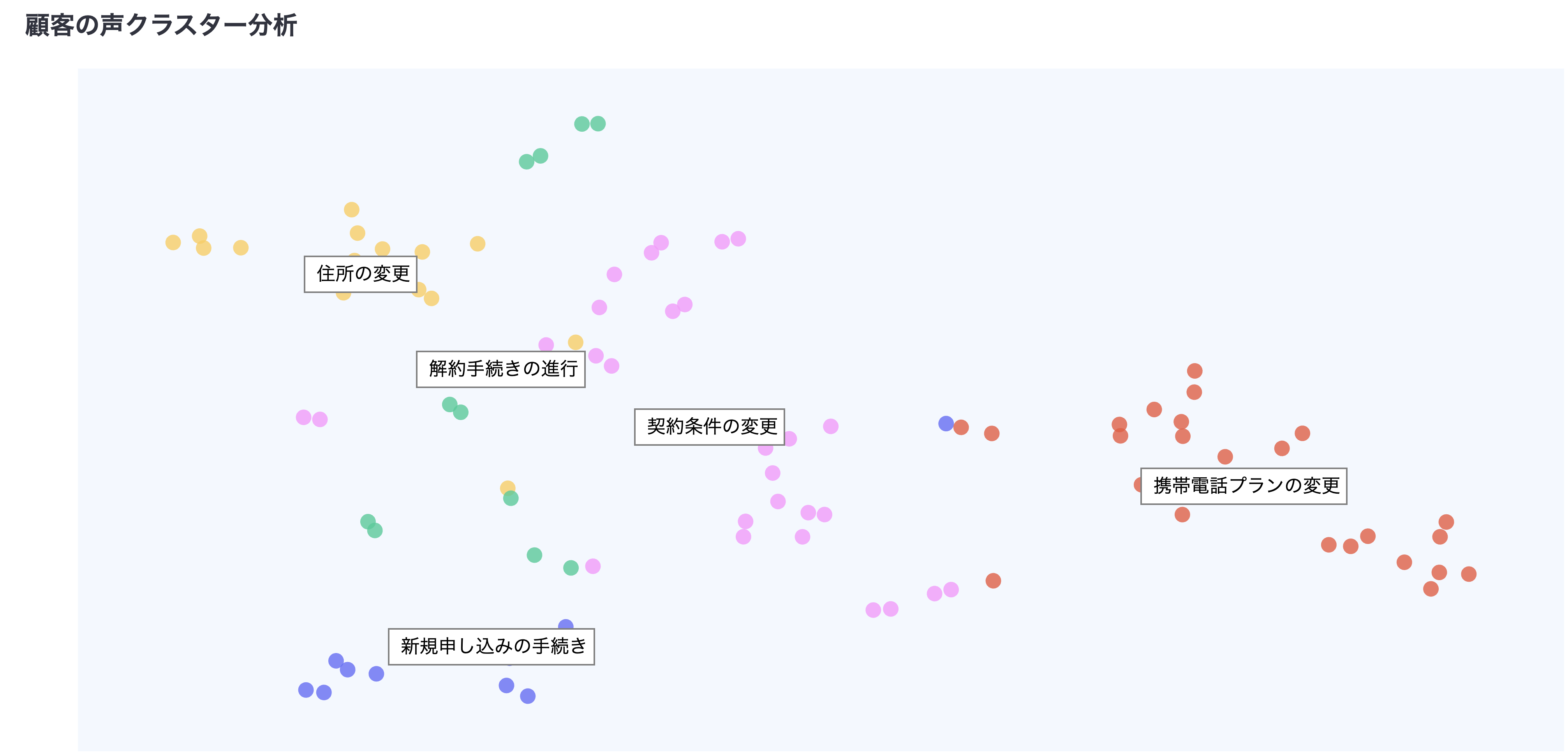
実行が完了するとクラスタが可視化できており、それぞれのクラスタ内の件数が棒グラフで表示されます。また、同じクラスタのテキストを確認すると似たような内容が同じクラスタに分類されていることが確認できますので次のステップに進みます。
ラベリング
極力人手を介さないで運用するため、グループ/クラスタにラベルをつけるステップもAIに実施してもらいます。こちらも本家の実装を参考にデータブリックスで実行できるように変更しています。ここでもLlama 3.3を使ってラベル付けします。
# Install the required packages
from tqdm import tqdm
import numpy as np
import pandas as pd
from databricks.sdk import WorkspaceClient
def labelling(config, plot_df):
results = pd.DataFrame()
sample_size = config['labelling']['sample_size']
prompt = config['labelling']['prompt']
model = config['labelling']['model']
question = config['question']
cluster_ids = plot_df['cluster'].unique()
for _, cluster_id in tqdm(enumerate(cluster_ids), total=len(cluster_ids)):
args_sample = plot_df[plot_df['cluster'] == cluster_id]['text'].values
args_sample = np.random.choice(args_sample, size=min(len(args_sample), sample_size), replace=False)
args_sample_outside = plot_df[plot_df['cluster'] != cluster_id]['text'].values
args_sample_outside = np.random.choice(args_sample_outside, size=min(len(args_sample_outside), sample_size), replace=False)
label = generate_label(question, args_sample, args_sample_outside, prompt, model)
results = pd.concat([results, pd.DataFrame([{'cluster-id': cluster_id, 'label': label}])], ignore_index=True)
return results
def generate_label(question, args_sample, args_sample_outside, prompt, model):
w = WorkspaceClient()
llm = w.serving_endpoints.get_open_ai_client()
outside = '\n * ' + '\n * '.join(args_sample_outside)
inside = '\n * ' + '\n * '.join(args_sample)
input_text = f"Question of the consultation: {question}\n\n" + \
f"Examples of arguments OUTSIDE the cluster:\n{outside}\n\n" + \
f"Examples of arguments INSIDE the cluster:\n{inside}"
response = llm.chat.completions.create(
messages=[{"role": "system", "content": prompt}, {"role": "user", "content": input_text}],
model=model,
max_tokens=256
)
return response.choices[0].message.content.strip()
# Config example
config = {
'output_dir': 'your_output_directory',
'labelling': {
'sample_size': 5,
'prompt': """あなたは、コンサルテーションの議論を分類するラベリングアシスタントです。ある議論のまとまり(クラスター)に対して、その内容を端的に表すラベルを1つ作成してください。クラスターの主な話題、関連する問い合わせのリスト、関係ない問い合わせのリストが与えられます。ラベルは以下のルールに従ってください:
・質問からすでに明らかな文脈は含めない
・「〜に関すること」「〜についての問い合わせ」「〜を行う」といった表現は使わない
・名詞で終わるのではなく、「〜の変更」「〜の依頼」など動詞を体言止めで終える
・簡潔であること
・クラスター内と外の問い合わせを正しく区別できるよう、十分な正確さをもつこと
回答はラベルのみを返してください。""",
'model': 'databricks-meta-llama-3-3-70b-instruct'
},
'question': 'これらの問い合わせの主なテーマは何か?'
}
# Run labelling
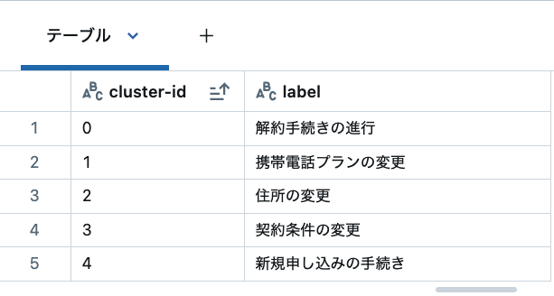
res = labelling(config, plot_df)
display(res)
結果を見るとトピックに重複もなく良い感じにカテゴリ分けしてくれていることがわかります。
spark.createDataFrame(res).write.mode("overwrite").saveAsTable(
    f"{CATALOG}.{SCHEMA}.{LABELS_TABLE}"
)
# Set the catalog and schema
spark.sql(f"USE CATALOG `{CATALOG}`")
spark.sql(f"USE SCHEMA `{SCHEMA}`")

# Create or replace the gold table by joining plot and labels tables
query = f"""
CREATE OR REPLACE TABLE {GOLD_TABLE} AS
SELECT
  a.x,
  a.y,
  a.cluster,
  a.text,
  b.label
FROM
  {PLOT_TABLE} a
  LEFT JOIN {LABELS_TABLE} b
  ON a.cluster = b.`cluster-id`
"""

spark.sql(query)
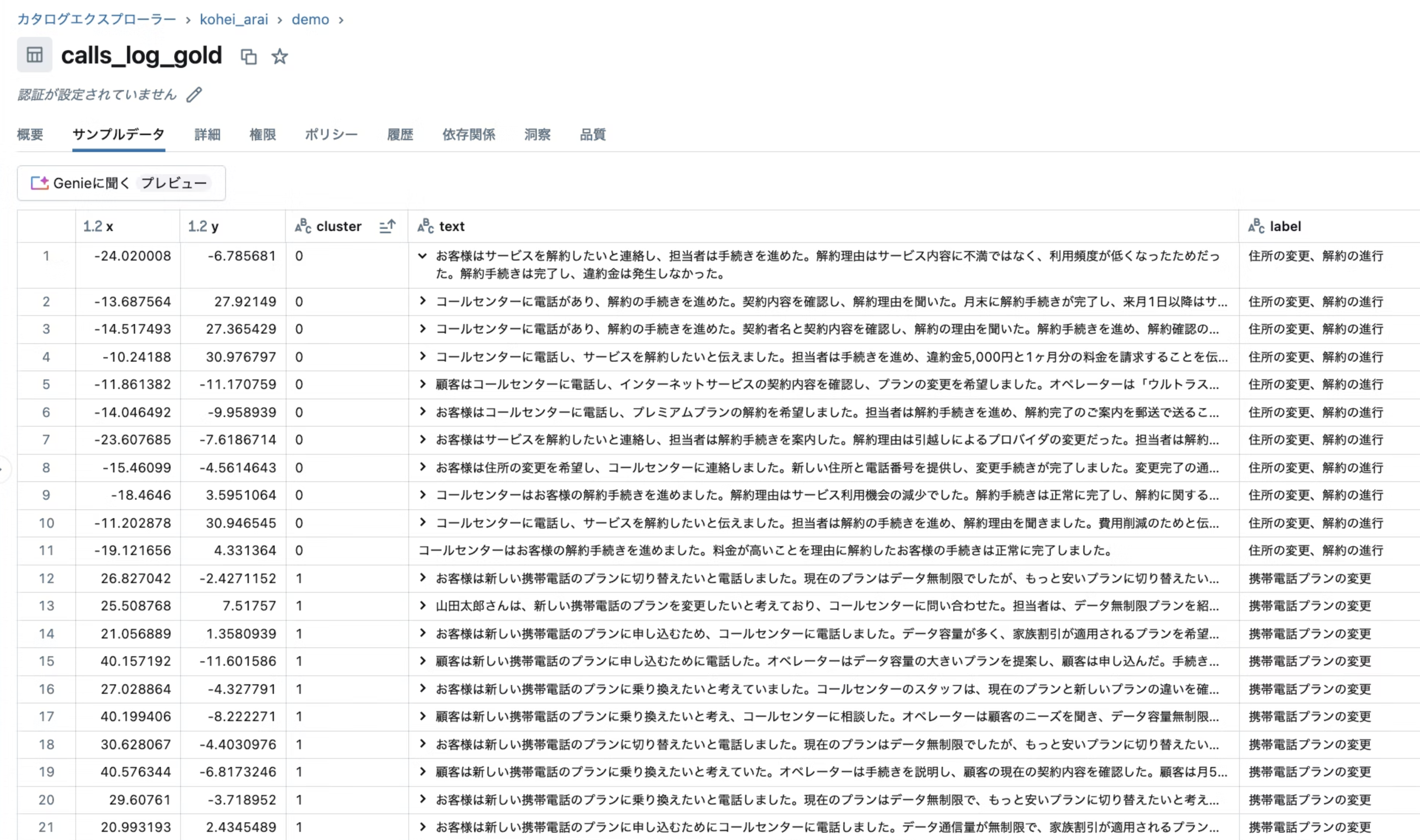
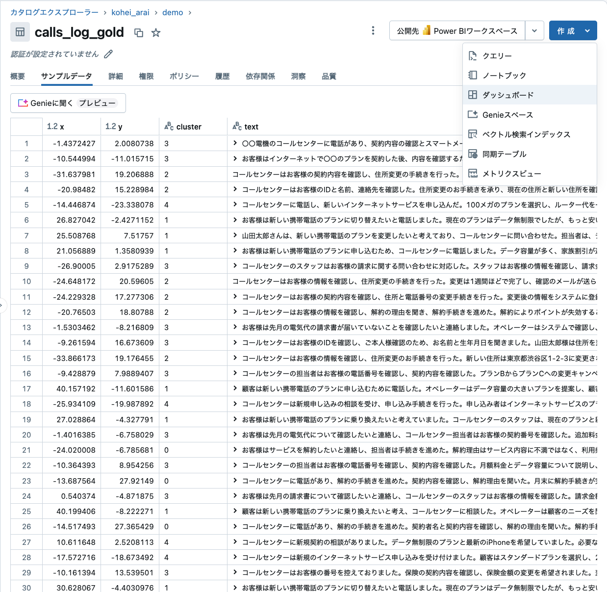
最終的に出来上がったテーブルを確認すると下記のようになっています。
x軸、y軸、クラスタとテキストの情報が存在します。これでデータ準備は完了ですので次のステップに進みます。
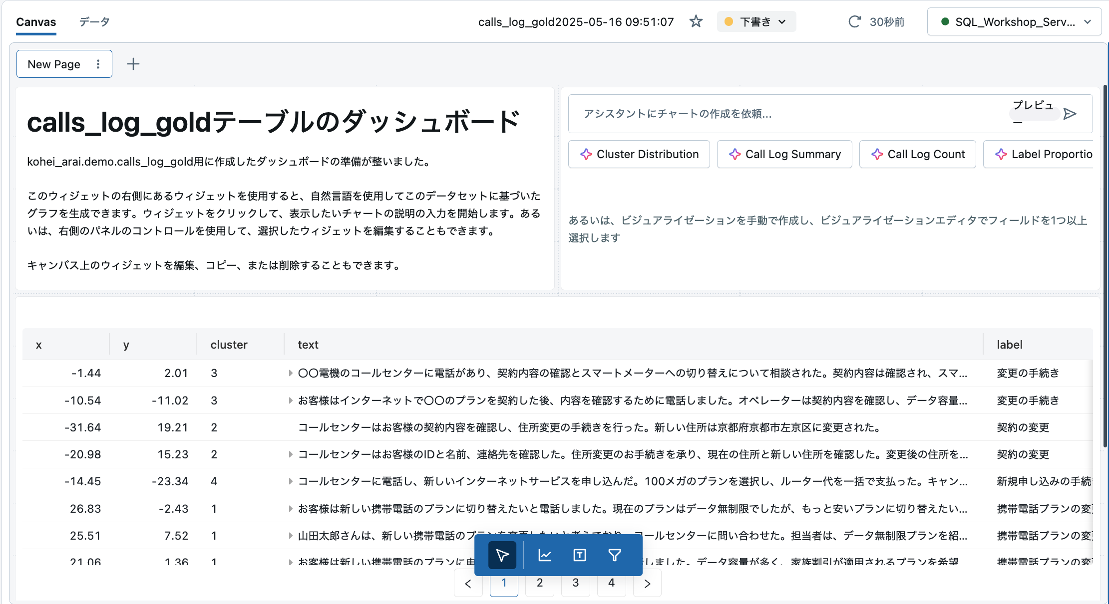
可視化
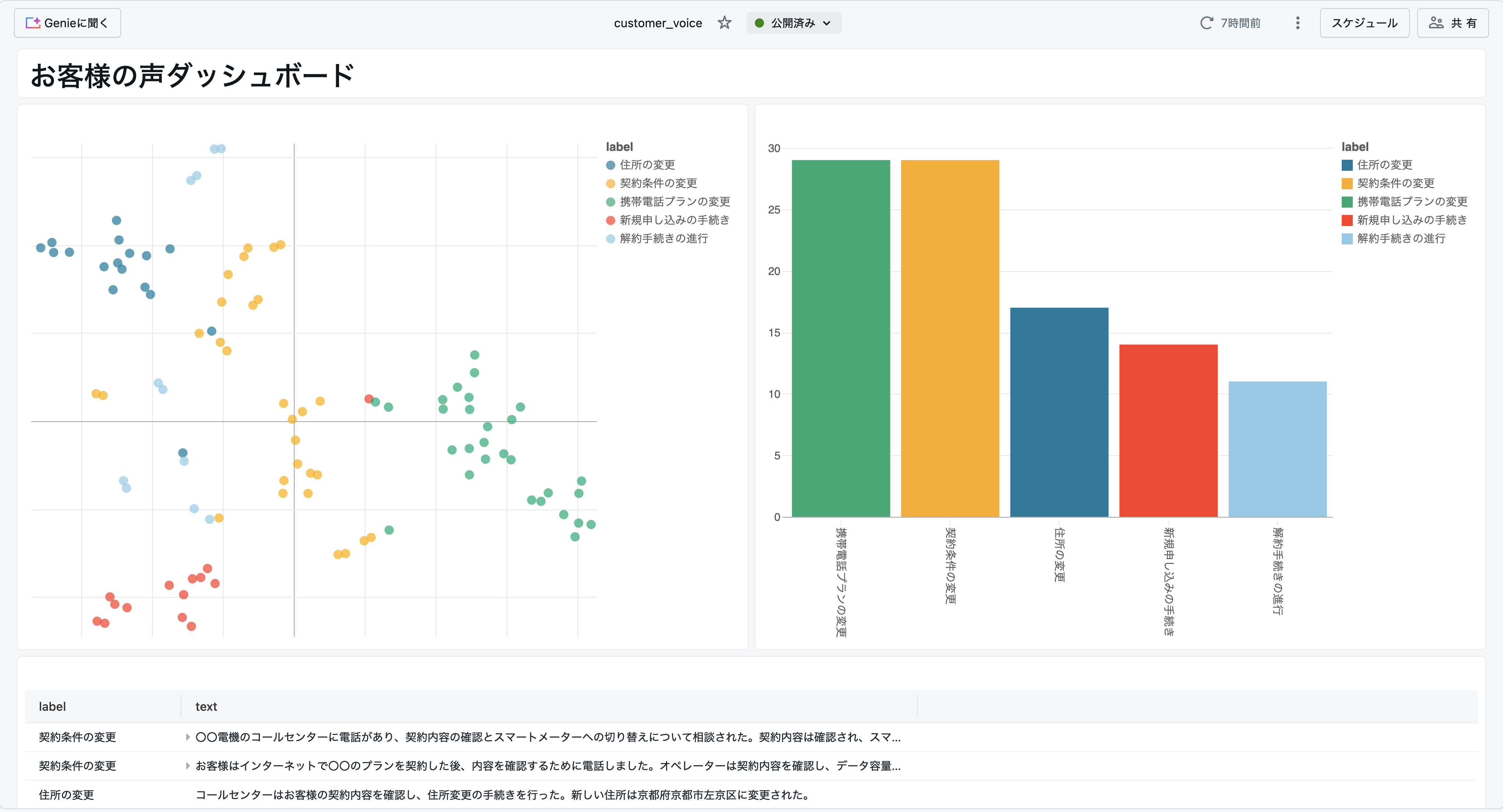
可視化は今回の記事のメイントピックではないので、簡単にご説明します。まずカタログエクスプローラーからテーブルを確認します。次に、右上の「ダッシュボード」をクリックします。
そうすると下図のようなダッシュボード画面が表示されるかと思います。
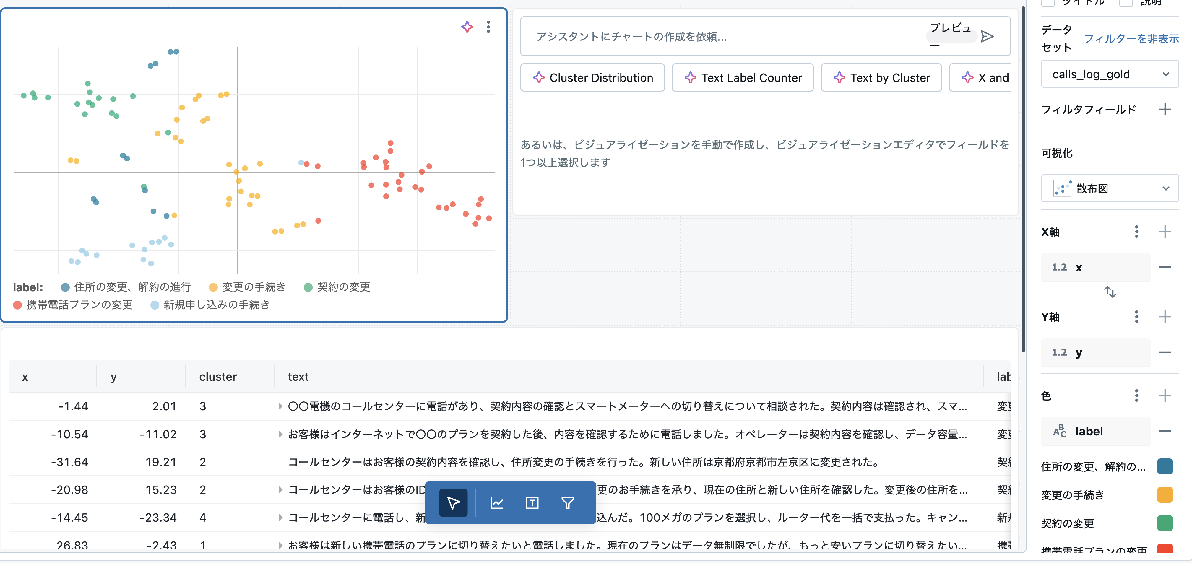
本記事の目的からは逸れるので説明は割愛しますが、ページ下部の「ビジュアライゼーションを追加」をクリックして、下図のように設定して作成します。
右上の可視化も同様に下図のように設定して作成します。
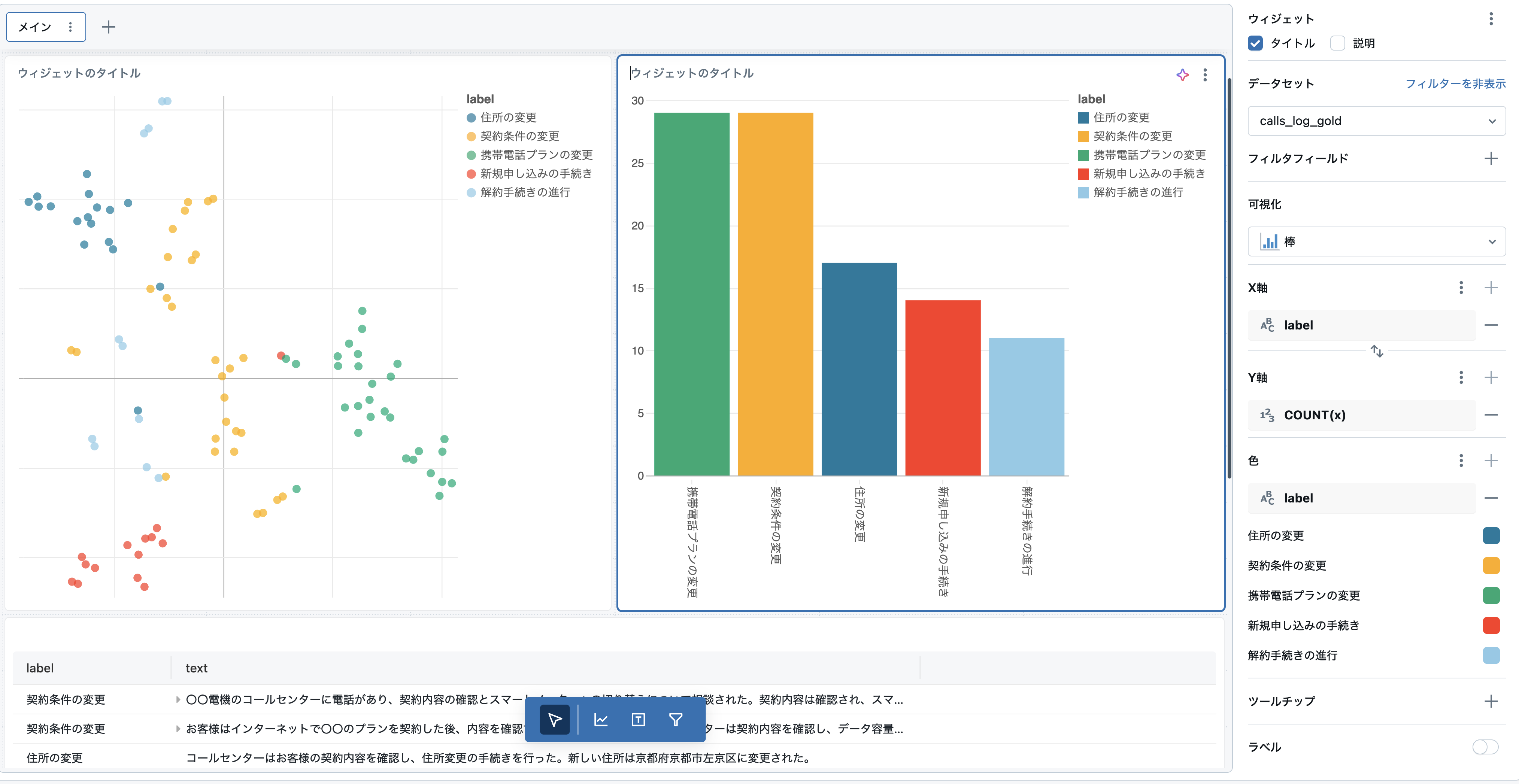
完了したら右上の「公開」をクリックします。皆さんにみていただける状態になるので完了です。ユーザに公開して業務に活用していただきましょう!
おまけの宣伝
最近弊社ではDatabricks Appsという機能を発表しており、こちらの機能を使うとStreamlitなどを使ったカスタムな可視化も可能です。(記事執筆時点では日本のリージョンでは利用不可)
おわりに
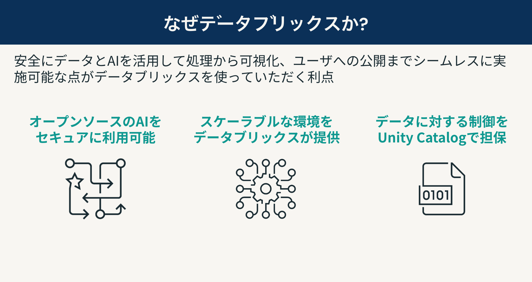
Databricksを使ってブロードリスニングを模倣したダッシュボードを作ってみましたが、いかがでしたでしょうか。皆さんの中で使ってみたいという方が一人でもいらっしゃったら嬉しいです。なんでわざわざデータブリックス?と思われた方に改めてデータブリックスを使っていただくメリットをお伝えすると下記かと思います。
- データブリックスがホストするオープンソースのモデルに簡単・セキュアにアクセス可能
- スケーラブルなETL処理・可視化の環境を提供
- カタログでダッシュボードやテーブルの権限管理可能
今回のユースケースを通じて
「こんな用途でも使える?」
「実装にあたって技術サポートもらえる?」
「コード全量が欲しいんだけど貰える?」
など疑問点やリクエストがあれば担当の営業チームや自分のTwitterやLinkedInまでご連絡ください。
また公式Twitterにも最新のプロダクト情報を投稿しているので、是非フォローしてください。
最後に今後も記事執筆を継続するモチベーションに繋がりますので「いいね」や記事の保存、SNSで共有いただけると嬉しいです。 宜しくお願いいたします!
参考リンク
ブロードリスニング:みんなが聖徳太子になる技術
https://note.com/nishiohirokazu/n/n15a60978113d