リーマン予想に興味ある人向け。
ワンチャン証明につながる可能性もあるかも。
2023.1.31 追記
※以下、複素関数論をある程度知っている前提。
勢いで書きなぐります。
$\xi(s)=\pi^{-\frac{s}{2}}\Gamma\left(\frac{s}{2}\right)\zeta(s)$に関して
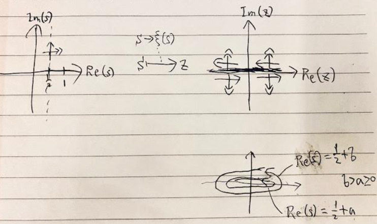
正則な複素関数の性質である等角写像の性質を使えば、クリティカルライン内で$Re(s)\neq 1/2$のとき$\xi(s)\neq0$を示せるのではないか。
$Re(s)=1/2$のとき$Im(\xi(s))=0$なので、$Re(s)=1/2$で実部を固定して$Im(s)$を増加させる動点的な線分を写像$s\to \xi(s)$で写した先は実軸上にある。
このとき、(十字にクロスするイメージで)実部を振った直行線分の写像先は実軸に直交するので、$Re(s)=1/2$の写像先の近傍ではその外側に写像される。
つまり、レムニスケートみたいに内側に交差することなく、横長な楕円1を描きながら零点$0$には触れずにぐるぐる回る。
これを同様に次の近傍(実部を1/2の外側に向かって振る)と、同じように外側に広がるはず。
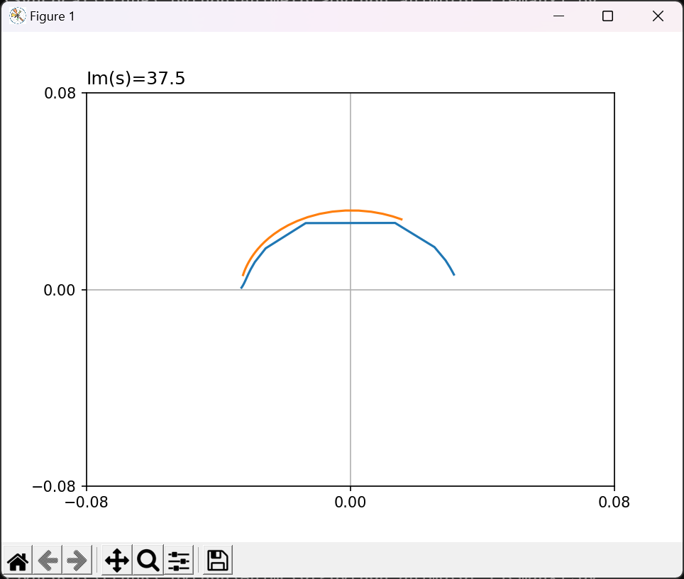
プロット
※対数的な補正を書けてます。(プログラム内参照)
プロット用ソースコード
import numpy as np
import matplotlib.pyplot as plt
from matplotlib import _pylab_helpers
import mpmath
mpmath.mp.dps = 14


def zeta_re_im(re,im_list):
    z_re = np.zeros(len(im_list))
    z_im = np.zeros(len(im_list))
    for i in range(len(im_list)):
        im = im_list[i]
        s = re + im*1j
        tmp = mpmath.zeta(s)*mpmath.gamma(0.5*s)*mpmath.power(mpmath.pi,-0.5*s)

        # 描画サイズを安定させるため変形をかける
        r = abs(tmp)
        tmp /= r
        tmp /= -mpmath.log(r)

        z_re[i] = tmp.real
        z_im[i] = tmp.imag
    return z_re,z_im

def pause_plot():
    s_im = np.arange(0, 1/2, 1/64) # 好みで変更。
    s_im += 5 # Im(s)の開始値. 好みで変更。
    fig, ax = plt.subplots(1, 1)

    s_re1 = 1/2 + 1/64
    s_re2 = 1/2 + 1/8

    x1,y1 = zeta_re_im(s_re1,s_im)
    x2,y2 = zeta_re_im(s_re2,s_im)

    lines1, = ax.plot(x1, y1) # ハンドル取得のため一度plot
    lines2, = ax.plot(x2, y2) # ハンドル取得のため一度plot
    # ax.plot([0,1], [0,0], linewidth=0.5) # x軸モドキを描画

    view_scale = 0.08
    ax.set_xlim(-view_scale, view_scale) # x軸の表示範囲を制限
    ax.set_ylim(-view_scale, view_scale) # y軸の表示範囲を制限
    ax.set_xticks([-view_scale,0,view_scale]) # x軸ticksを0,0.5,1の位置に設定
    ax.set_yticks([-view_scale,0,view_scale]) # x軸ticksを0,0.5,1の位置に設定
    ax.grid()

    # ここから無限にplotする
    while True:
        # グラフウィンドウを閉じられたらプログラムを終了する
        manager = _pylab_helpers.Gcf.get_active()
        if manager is None: break

        s_im += .5 # 好みで変更
        x1,y1 = zeta_re_im(s_re1,s_im) # plot対象関数の計算
        x2,y2 = zeta_re_im(s_re2,s_im) # plot対象関数の計算

        lines1.set_data(x1, y1)
        lines2.set_data(x2, y2)

        ax.set_title("Im(s)="+str(s_im[0]),loc='left')

        # 次の描画までの待ち時間(秒)
        plt.pause(.05)

if __name__ == "__main__":
    pause_plot()
以下、最初に投稿したときの内容
やったこと
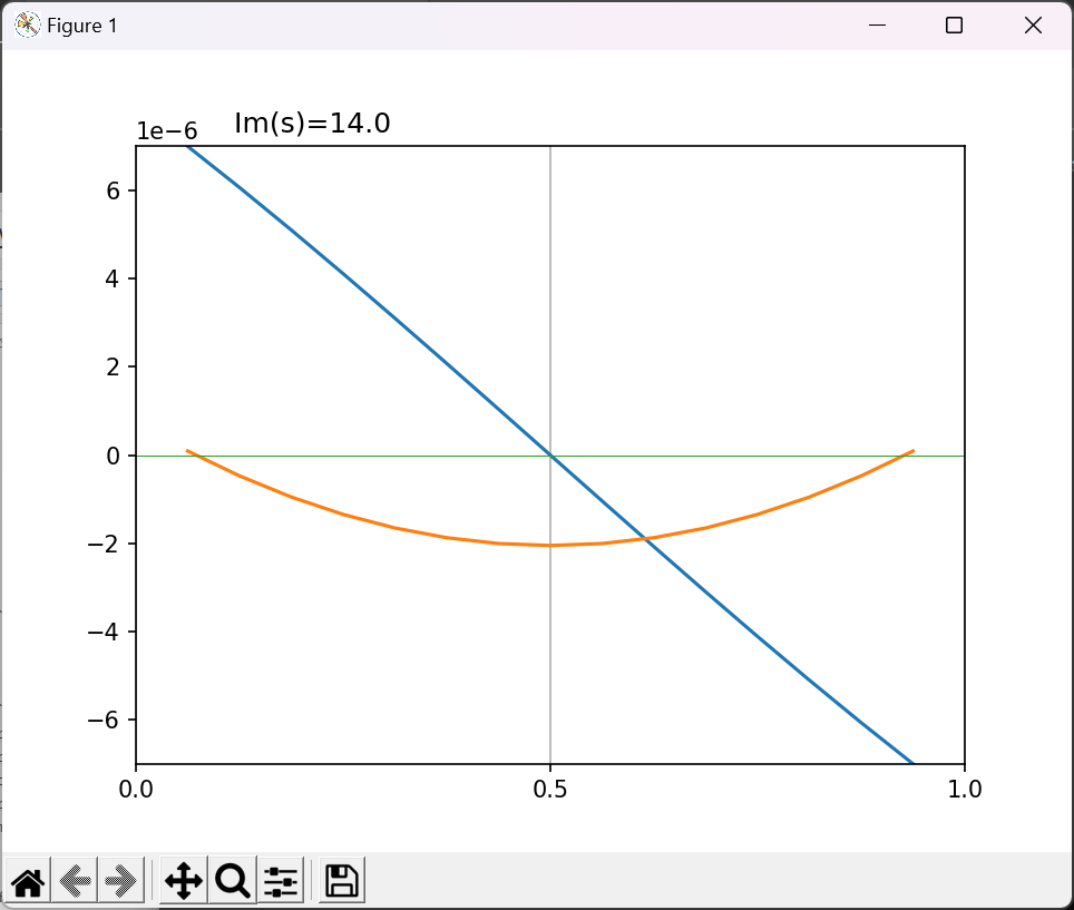
リーマンのゼータ関数を対称形($f(s)=f(1-s)$)になるように変形した関数
$\xi(s)=\pi^{-\frac{s}{2}}\Gamma\left(\frac{s}{2}\right)\zeta(s)$
をプロットしている。
$Re(s)=\frac{1}{2}$付近を、$Im(s)$を時間経過にしたがって増加させて$\xi(s)$の実部と虚部をプロットしてみた。(クリティカルラインを上っていくイメージ)
ソースコード
実部と虚部を同じエリアにプロットするバージョン
import numpy as np
import matplotlib.pyplot as plt
from matplotlib import _pylab_helpers
import mpmath
mpmath.mp.dps = 12


def zeta_re_im(re_list,im):
    z_re = np.zeros(len(re_list))
    z_im = np.zeros(len(re_list))
    for i in range(len(re_list)):
        s = re_list[i] + im*1j
        tmp = mpmath.zeta(s)*mpmath.gamma(0.5*s)*mpmath.power(mpmath.pi,-0.5*s)
        z_re[i] = tmp.real
        z_im[i] = tmp.imag
    return z_re,z_im

def pause_plot():
    t = 1 # 好みで変更。値が大きいほどzeta_re_imの計算速度が低下する。840以上あたりで結果の値が小さすぎて波形が見えなくなる。
    fig, ax = plt.subplots(1, 1)

    x = np.arange(1/16, (16-1+1)/16, 1/16) # 好みで変更。x方向の点の始点,終点(端点を含まない),刻み

    y1,y2 = zeta_re_im(x,t)

    ax.set_xticks([0,0.5,1]) # x軸ticksを0,0.5,1の位置に設定
    lines1, = ax.plot(x, y1) # ハンドル取得のため一度plot
    lines2, = ax.plot(x, y2) # ハンドル取得のため一度plot
    ax.plot([0,1], [0,0], linewidth=0.5) # x軸モドキを描画

    ax.set_xlim( 0, 1) # x軸の表示を[0,1]に制限
    ax.set_ylim(-2, 2) # dummy
    ax.grid(axis="x") # 縦方向のグリッドを表示

    # ここから無限にplotする
    while True:
        # グラフウィンドウを閉じられたらプログラムを終了する
        manager = _pylab_helpers.Gcf.get_active()
        if manager is None: break

        t += 1/8 # 好みで変更
        y1,y2 = zeta_re_im(x,t) # plot対象関数の計算

        lines2.set_data(x, y1) # Re part # lines1, lines2 が入れ替わっているのはタイポ・・ キャプチャした後なのでそのままにします
        lines1.set_data(x, y2) # Im part

        # 左側にy軸の指数部が出てくるので空白を入れてかぶらないようにしている
        ax.set_title("           Im(s)="+str(t),loc='left')

        tmp_abs_max = max(abs(y1.min()),abs(y1.max()),abs(y2.min()),abs(y2.max()))
        ax.set_ylim((-tmp_abs_max, tmp_abs_max))

        # 次の描画までの待ち時間(秒)
        plt.pause(.05)

if __name__ == "__main__":
    pause_plot()
実部と虚部でグラフを分離したバージョン
import numpy as np
import matplotlib.pyplot as plt
from matplotlib import _pylab_helpers
import mpmath
mpmath.mp.dps = 12


def zeta_re_im(re_list,im):
    z_re = np.zeros(len(re_list))
    z_im = np.zeros(len(re_list))
    for i in range(len(re_list)):
        s = re_list[i] + im*1j
        tmp = mpmath.zeta(s)*mpmath.gamma(0.5*s)*mpmath.power(mpmath.pi,-0.5*s)
        z_re[i] = tmp.real
        z_im[i] = tmp.imag
    return z_re,z_im

def pause_plot():
    t = 1 # 好みで変更。値が大きいほどzeta_re_imの計算速度が低下する。840以上あたりで結果の値が小さすぎて波形が見えなくなる。
    fig, axes = plt.subplots(2, 1) # 縦に2個描画エリアを確保

    x = np.arange(1/16, (16-1+1)/16, 1/16) # 好みで変更。x方向の点の始点,終点(端点を含まない),刻み

    y1,y2 = zeta_re_im(x,t)

    axes[0].set_xticks([0,0.5,1]) # x軸ticksを0,0.5,1の位置に設定
    axes[1].set_xticks([0,0.5,1])
    lines1, = axes[0].plot(x, y1) # ハンドル取得のため一度plot
    lines2, = axes[1].plot(x, y2)
    axes[0].plot([0,1], [0,0], linewidth=0.5) # x軸モドキを描画
    axes[1].plot([0,1], [0,0], linewidth=0.5)

    axes[0].set_xlim( 0, 1) # x軸の表示を[0,1]に制限
    axes[1].set_xlim( 0, 1)
    axes[0].set_ylim(-2, 2) # dummy
    axes[1].set_ylim(-2, 2)
    axes[0].grid(axis="x") # 縦方向のグリッドを表示
    axes[1].grid(axis="x")

    # ここから無限にplotする
    while True:
        # グラフウィンドウを閉じられたらプログラムを終了する
        manager = _pylab_helpers.Gcf.get_active()
        if manager is None: break

        t += 1/8 # 好みで変更
        y1,y2 = zeta_re_im(x,t) # plot対象関数の計算

        lines1.set_data(x, y1) # Re part
        lines2.set_data(x, y2) # Im part

        # 左側にy軸の指数部が出てくるので空白を入れてかぶらないようにしている
        axes[1].set_title("           Im(s)="+str(t),loc='left')

        tmp_abs_max = max(abs(y1.min()),abs(y1.max()))
        axes[0].set_ylim((-tmp_abs_max, tmp_abs_max))

        tmp_abs_max = max(abs(y2.min()),abs(y2.max()))
        axes[1].set_ylim((-tmp_abs_max, tmp_abs_max))

        # 次の描画までの待ち時間(秒)
        plt.pause(.02)

if __name__ == "__main__":
    pause_plot()
画面キャプチャ

参考記事 - プロット関連
プロットに関するベース部分はほぼ下記の記事をもとにしています。
参考サイト
-
実際にはIm(s)を大きくすると\xi(s)の絶対値が指数関数的に小さくなっていくので、インボリュート曲線的な感じになる(?) ↩