量子化とは?
関数を離散化してNbitで表し、コンピュータに解析させることができる形にすることです。量子力学の「量子」も、もともとは離散化することからきています。今回実装していくもの
具体的に$ cosx $関数をBbitであらわして、実際にグラフがどうなるのかを見ていきます。前準備としては下のような形です。
- サンプリング周期を$ \tau $とし関数を$ f(n\tau) = x $でサンプリングします
- $ B $bitつかい線形量子化します。($ i = 1, 2, \cdots , 2^B = N $)
- $ x_i < x < x_{i + 1} $のときは $ \bar{x_i} $とします($ \bar{x_i} = \frac{x_{i + 1} + x_i}{2} $)<\li>
実装
``` import numpy as np import matplotlib.pyplot as plt import cmath import bisectcosxを量子化してみる
t = 0.01 #サンプリング周期
max_x = 1
min_x = -1
B = 3 #使用するBit数
x_barを計算して配列に格納
X = []
for i in range(2 ** B):
x_pre = min_x + (i / (2 ** B)) * abs(max_x - min_x)
x_nex = min_x + (i + 1) / (2 ** B) * abs(max_x - min_x)
x_bar = (x_pre + x_nex) / 2
X.append(x_bar)
サンプリングした値を量子化する
cosxは一周期
T = 2 * np.pi
量子化した後のデータ
x = []
y = []
for i in np.arange(0, T, t):
x_sample = np.cos(i)
#xに一番近い値を二分探索で求める
index = bisect.bisect(X, x_sample)
x.append(i)
if index == 0:
y.append(X[index])
elif index == 2 ** B:
y.append(X[index - 1])
else:
#xと距離が近いほうの値を採用する。
x_front_dis = abs(x_sample - X[index - 1])
x_back_dis = abs(x_sample - X[index])
if x_front_dis < x_back_dis:
y.append(X[index - 1])
else:
y.append(X[index])
量子化する前とした後のグラフは次のようになります。

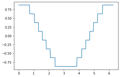
bitの数を増やせばもときれいに近似できます。