MCMCのスクラッチ実装をMultiprocessing化で高速化してみる記事です。
先日の記事、「【統計学】マルコフ連鎖モンテカルロ法(MCMC)によるサンプリングをアニメーションで解説してみる。」では、chainを実装していなかったので、1つのchainのみでしたが、これを複数chainでサンプリングを行い、かつマルチプロセスとして実行できるようにしてみました。MCMCはchain毎に独立しているので、単にプロセスをわけるだけでOKなので簡単に高速化できました。
環境
- OSX Yosemite 10.10.5
- Python 2.7
- Anaconda 3.18.9
- CPU: 1.2GHz デュアルコアIntel Core Mプロセッサ
- MacBook (Retina, 12-inch, Early 2015)
⇒ 2コアなので、2プロセスまでしか有効に高速化できません・・・
本記事のコード
GitHubにコードを掲載しています。
https://github.com/matsuken92/Qiita_Contents/blob/master/multiprocessing/parallel_MCMC.ipynb
MultiProcessingの基本
まずは簡単な処理で、MultiProcessingの動きを見ていきたいと思います。
まずはライブラリのインポートです。Poolという複数のワーカープロセスをマネジメントするクラスを使います。
from multiprocessing import Pool
とりあえずなんか重そうな処理ということで、たくさんループする処理をターゲットにしてみます。足し算するだけですが、100000000回くらいまわすと数秒かかります。
def test_calc(num):
    """重い処理"""
    _sum = 0
    for i in xrange(num):
        _sum += i
    return _sum
この処理を順番に2回実行した時のスピードを計測してみます。
# シーケンシャルに2回実行した時の時間を計測
start = time.time()
_sum = 0
for _ in xrange(2):
    _sum += test_calc(100000000)
end = time.time()
print _sum
print "time: {}".format(end-start)
12秒弱かかりました。
9999999900000000
time: 11.6906960011
次に、2プロセス並列で同じ処理を行い、計測してみます。
# 2プロセスで実行した時の時間を計測
n_worker = 2

pool = Pool(processes=n_worker)

# 2つのプロセスが実行する関数に渡す引数リスト
args = [100000000] * n_worker

start = time.time() # 計測
result = pool.map(test_calc, args)
end = time.time()   # 計測

print  np.sum(result)
print "time: {}".format(end-start)
pool.close()
6秒少々なので、半分近くの時間で完了です。2プロセスによる高速化が出来ました ![]()
9999999900000000
time: 6.28346395493
MCMCサンプリングへのMultiProcessingの適用
さて、これをMCMCサンプリングの各chainを並列に処理することに応用してみます。
毎回のことですが、まずはライブラリのインポートです
import numpy as np
import numpy.random as rd
import scipy.stats as st
import copy, time, os
from datetime import datetime as dt

from multiprocessing import Pool

%matplotlib inline
import matplotlib.pyplot as plt
import seaborn as sns
sns.set(style="whitegrid", palette="muted", color_codes=True)
関数P(・)はターゲットにする事後分布のカーネルです。ここでは2次元正規分布のカーネルを使用しています。
# 確率関数から正規化定数を除いたもの
def P(x1, x2, b):
    assert np.abs(b) < 1
    return np.exp(-0.5*(x1**2 - 2*b*x1*x2 + x2**2))
提案分布のパラメーターをグローバルとして定義しています。
また、時間計測用のnow(・)関数も定義します。現在時刻の文字列を表示する関数です。
# global parameters
b = 0.5
delta = 1

def now():
    return  dt.strftime(dt.now(), '%H:%M:%S')
次が、サンプリングを実行する関数です。指定したサンプル数に達するまでサンプリングを行います。関数化されて、時間測定のコードが追加されている以外はほとんど前回と変わりません。
この関数を並列実行させるところがキモですね。chain毎のサンプリングなので、プロセス間で独立に動いて良いので、特にプロセス間通信も不要で楽チンな感じです。
def exec_sampling(n_samples):
    global b, delta
    rd.seed(int(time.time())+os.getpid())
    pid = os.getpid()
    start = time.time()
    start_time = now()

    #initial state
    sampling_result = []
    current = np.array([5, 5])
    sampling_result.append(current)
    cnt = 1
    while cnt < n_samples:
        # rv from proposal distribution(Normal Dist: N(0, delta) )
        next = current + rd.normal(0, delta, size=2)
        r = P(next[0], next[1], b)/P(current[0], current[1], b)

        if r > 1 or r > rd.uniform(0, 1):
            # 0-1の一様乱数がrより大きい時は状態を更新する。
            current = copy.copy(next)
            sampling_result.append(current)
            cnt += 1

    end = time.time()
    end_time = now()

    # 各chain毎の所要時間の表示
    print "PID:{}, exec time: {}, {}-{}".format(pid, end-start, start_time, end_time)
    return sampling_result
下記の3つの関数draw_scatter ()、draw_traceplot ()、remove_burn_in_samples()はサンプリング結果を処理する関数です。
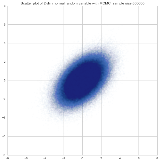
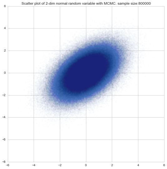
def draw_scatter(sample, alpha=0.3):
"""サンプリング結果の散布図を描画"""
plt.figure(figsize=(9,9))
plt.scatter(sample[:,0], sample[:,1], alpha=alpha)
plt.title("Scatter plot of 2-dim normal random variable with MCMC. sample size:{}".format(len(sample)))
plt.show()
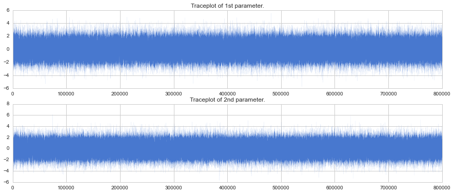
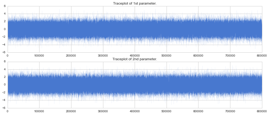
def draw_traceplot(sample):
"""サンプリング結果のtraceplotを描画"""
assert sample.shape[1] == 2
plt.figure(figsize=(15, 6))
for i in range(2):
plt.subplot(2, 1, i+1)
plt.xlim(0, len(sample[:,i]))
plt.plot(sample[:,i], lw=0.05)
if i == 0:
order = "1st"
else:
order = "2nd"
plt.title("Traceplot of {} parameter.".format(order))
plt.show()
def remove_burn_in_samples(total_sampling_result, burn_in_rate=0.2):
"""Burn-inに指定されている区間のサンプルを除外する。"""
adjust_burn_in_result = []
for i in xrange(len(total_sampling_result)):
idx = int(len(total_sampling_result[i])*burn_in_rate)
adjust_burn_in_result.extend(total_sampling_result[i][idx:])
return np.array(adjust_burn_in_result)
下記が、並列処理を行っている関数です。よく見ると最初の簡易的な例と実質ほとんど変わらないことがわかります。
def parallel_exec(n_samples, n_chain, burn_in_rate=0.2):
    """並列処理の実行"""

    # 1chainあたりのサンプルサイズを算出
    n_samples_per_chain = n_samples / float(n_chain)
    print "Making {} samples per {} chain. Burn-in rate:{}".format(n_samples_per_chain, n_chain, burn_in_rate)

    # Poolオブジェクトの作成
    pool = Pool(processes=n_chain)

    # 実行用の引数の生成
    n_trials_per_process = [n_samples_per_chain] * n_chain

    # 並列処理の実行
    start = time.time() # 計測
    total_sampling_result = pool.map(exec_sampling, n_trials_per_process)
    end = time.time()   # 計測

    # トータル所要時間の表示
    print "total exec time: {}".format(end-start)

    # Drawing scatter plot
    adjusted_samples = remove_burn_in_samples(total_sampling_result)
    draw_scatter(adjusted_samples, alpha=0.01)
    draw_traceplot(adjusted_samples)
    pool.close()
さて、実際の効果を見てみましょう。サンプリング数:1,000,000で、chain数が2の場合と1の場合を計測します。
サンプリング数: 1,000,000, chain数: 2
# パラメーター: n_samples = 1000000, n_chain = 2
parallel_exec(1000000, 2)
1ワーカープロセスあたり12秒ほど、計19秒弱でサンプリング完了しています。
Making 500000.0 samples per 2 chain. Burn-in rate:0.2
total exec time: 18.6980280876
PID:2374, exec time: 12.0037689209, 20:53:41-20:53:53
PID:2373, exec time: 11.9927477837, 20:53:41-20:53:53
サンプリング数: 1,000,000, chain数: 1
# パラメーター: n_samples = 1000000, n_chain = 1
parallel_exec(1000000, 1)
1つのワーカープロセスで実行すると、33秒弱でした。なので、2つのプロセスで実行すると1.7倍ほど早く実行できていることがわかります ![]()
Making 1000000.0 samples per 1 chain. Burn-in rate:0.2
total exec time: 32.683218956
PID:2377, exec time: 24.7304420471, 20:54:07-20:54:31
参考
Python Documentation(2.7ja1) 16.6. multiprocessing — プロセスベースの “並列処理” インタフェース
http://docs.python.jp/2.7/library/multiprocessing.html
ハイパフォーマンスPython(オライリー)
https://www.oreilly.co.jp/books/9784873117409/