ゲート方式の量子コンピュータで半加算器を作ったメモ

以下のドキュメントを参考にQiskitを使ったゲート方式の量子コンピュータの勉強メモです。

QiskitはPythonのモジュールです。Condaがインストールされていれば、pipでインストールすることができます。

conda create -n qiskit python=3.8
conda activate qiskit
pip install jupyter matplotlib pylatexenc qiskit

半加算器を量子ゲートで組んでみる

2量子ビットの加算を行う。パターンとしては以下の通り。
0 + 0 = 00
1 + 0 = 01
0 + 1 = 01
1 + 1 = 10
今回の量子回路は、入力に2量子ビット、出力に2量子ビット使うため、合計4量子ビットを用意する。
回路の手前2つのCNOT(cx)は1桁目の加算回路。CNOTは制御量子ビット（今回は入力）が1の場合だけ出力（今回は出力の1桁目）のビットを反転する。 3つ目のToffoli(ccx)は2つの量子ビットのAND結果が出力（今回は出力の2桁目）になる。
以下は、入力を1と1とした場合。

# 4量子ビット、測定した結果は2つの量子回路を作成
qc_ha = QuantumCircuit(4,2)
# 入力値設定
qc_ha.x(0) # 1を設定（初期値が0なので1になる）
qc_ha.x(1) # 1を設定（初期値が0なので1になる）
# 回路
qc_ha.barrier()
qc_ha.cx(0,2)
qc_ha.cx(1,2)
qc_ha.ccx(0,1,3)
qc_ha.barrier()
# 結果計測
qc_ha.measure(2,0)
qc_ha.measure(3,1)
qc_ha.draw(output='mpl')

計算してみる。

sim = Aer.get_backend('aer_simulator')
counts = sim.run(qc_ha, shots=1000).result().get_counts()
# ヒストグラムで測定された確率をプロット
plot_histogram(counts)

入力が1と1なので、結果は10になる。入力を変える場合は、入力値設定箇所をコメントにする。

重ね合わせ状態の入力を半加算器に入れてみる

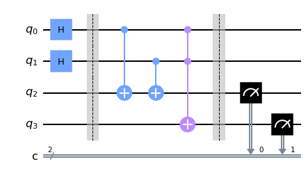
量子コンピューターらしくないので、入力をアダマールゲートで0と1の状態を確率50%の重ね合わせ状態にしてみる。

qc_ha = QuantumCircuit(4,2)
# 入力値設定
qc_ha.h(0) # Hゲートで確立0.5の重ね合わせ状態を設定
qc_ha.h(1) # Hゲートで確立0.5の重ね合わせ状態を設定
# 回路
qc_ha.barrier()
qc_ha.cx(0,2)
qc_ha.cx(1,2)
qc_ha.ccx(0,1,3)
qc_ha.barrier()
# 結果計測
qc_ha.measure(2,0)
qc_ha.measure(3,1)
qc_ha.draw(output='mpl')

計算してみる。

sim = Aer.get_backend('aer_simulator')
# 1000回ショット
counts = sim.run(qc_ha, shots=1000).result().get_counts()
# ヒストグラムで測定された確率をプロット
plot_histogram(counts)

入力の量子ビットが0もしくは1となるため、01の出力は00や10と比べて約2倍になる。
0 + 0 = 00
1 + 0 = 01
0 + 1 = 01
1 + 1 = 10

もっと実行回数を多くすればちゃんと2倍になる。

sim = Aer.get_backend('aer_simulator')
# 1000000回ショット
counts = sim.run(qc_ha, shots=1000000).result().get_counts()
# ヒストグラムで測定された確率をプロット
plot_histogram(counts)

ちなみに、一回だけ実行した場合の結果も書いておく。

sim = Aer.get_backend('aer_simulator')
# 1回ショット
counts = sim.run(qc_ha, shots=1).result().get_counts()
# ヒストグラムで測定された確率をプロット
plot_histogram(counts)

結果は実行するたびに、00は25%、10は50%、11は25%の確立で測定される。（実行するたびに結果が変わる）

バックエンドを変更してみる

シミュレーターを変更することもできる。以下のコマンドでバックエンドをリスト表示できる。
バックエンドは以下のURLを参考にしてください。
https://qiskit.org/documentation/locale/ja_JP/tutorials/simulators/1_aer_provider.html

Aer.backends()

バックエンドのリスト

[AerSimulator('aer_simulator'),
 AerSimulator('aer_simulator_statevector'),
 AerSimulator('aer_simulator_density_matrix'),
 AerSimulator('aer_simulator_stabilizer'),
 AerSimulator('aer_simulator_matrix_product_state'),
 AerSimulator('aer_simulator_extended_stabilizer'),
 AerSimulator('aer_simulator_unitary'),
 AerSimulator('aer_simulator_superop'),
 QasmSimulator('qasm_simulator'),
 StatevectorSimulator('statevector_simulator'),
 UnitarySimulator('unitary_simulator'),
 PulseSimulator('pulse_simulator')]

QASMシミュレーターに変更。

sim = Aer.get_backend('qasm_simulator')
# 1000回ショット
counts = sim.run(qc_ha, shots=1000).result().get_counts()
# ヒストグラムで測定された確率をプロット
plot_histogram(counts)

シミュレーターのrun以外だと、executeで実行することもできる。

# executeを使う場合の書き方もある
sim = Aer.get_backend('qasm_simulator')
# 1000回ショット
job = execute(qc_ha, backend=sim, shots=1000)
result = job.result()
counts = result.get_counts(qc_ha)
# カウントされた結果をプリント
print(counts)
# ヒストグラムで測定された確率をプロット
plot_histogram( counts )

今回のメモは、これで終わりです。