「Rによる機械学習」の勉強履歴（4）

Rによる機械学習

（ソフトウェア品質技術者のための）データ分析勉強会で、書籍『Rによる機械学習 （Machine Learning with R）』を使用して機械学習を学ぶ。
https://www.amazon.co.jp/dp/4798145114/

第6章 数値データの予測 - 回帰法

用語

• 依存変数=目的変数
• 独立変数=説明変数
• 回帰木 : 予測結果は平均値で出す
• モデル木 : 予測結果は回帰式で出す

challenger.csvの分析

データの説明

• distress_ct : Oリングの異常数
• temperature : 気温（華氏）
• field_check_pressure : 実地点気圧
• flight_num : 発射ID

challenger.csvのdistress_ct（Oリングの異常数）は、順序尺度に近い分布を示していて、単回帰分析の目的変数としては、よくないかも。

散布図

> launch <- read_csv("challenger.csv")
Parsed with column specification:
cols(
  distress_ct = col_double(),
  temperature = col_double(),
  field_check_pressure = col_double(),
  flight_num = col_double()
)
> plot(launch)

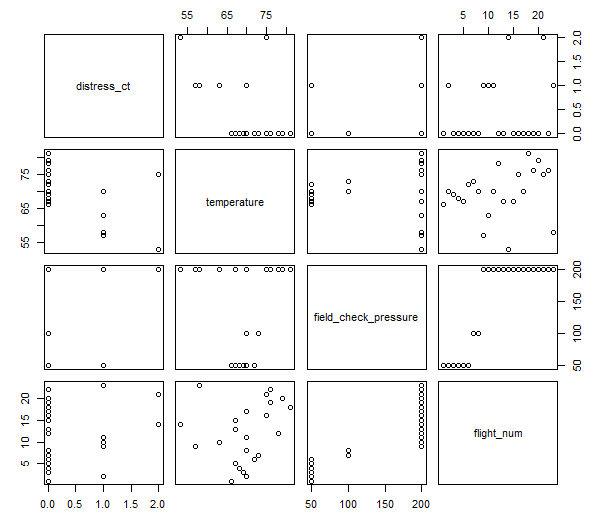
散布図を見るとtemperatureとdistress_ctの間に、なんとなく相関があるように見える。

相関係数

相関係数を求めてみる。

> cor(launch$temperature, launch$distress_ct)
[1] -0.5111264

相関係数の使い方・注意点
https://atarimae.biz/archives/7966

重回帰分析

自分で作った回帰関数を使う

> reg <- function(y, x) {
+     x <- as.matrix(x)
+     x <- cbind(Intercept = 1, x)
+     b <- solve(t(x) %*% x) %*% t(x) %*% y
+     colnames(b) <- "estimate"
+     print(b)
+     }
> reg(y = launch$distress_ct, x = launch[2])
               estimate
Intercept    3.69841270
temperature -0.04753968
> reg(y = launch$distress_ct, x = launch[2:4])
                         estimate
Intercept             3.527093383
temperature          -0.051385940
field_check_pressure  0.001757009
flight_num            0.014292843

insurance.csvの分析

散布図行列

> install.packages("psych")
> library(psych)
> insurance<- read_csv("insurance.csv")
Parsed with column specification:
cols(
  age = col_double(),
  sex = col_character(),
  bmi = col_double(),
  children = col_double(),
  smoker = col_character(),
  region = col_character(),
  expenses = col_double()
)
> pairs.panels(insurance[c("age", "bmi", "children", "expenses")])

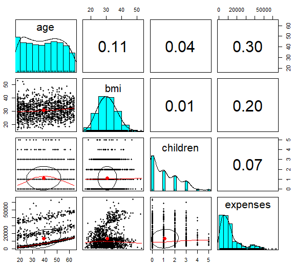
赤い点は、x,y軸の平均を示している。
楕円は、相関楕円で、相関の強さを可視化している。

重回帰分析

lm()関数を使う

> ins_model <- lm(expenses ~ ., data = insurance)
> summary(ins_model)

Call:
lm(formula = expenses ~ ., data = insurance)

Residuals:
     Min       1Q   Median       3Q      Max 
-11302.7  -2850.9   -979.6   1383.9  29981.7 

Coefficients:
                    Estimate Std. Error t value Pr(>|t|)    
(Intercept)         -11941.6      987.8 -12.089  < 2e-16 ***
age                    256.8       11.9  21.586  < 2e-16 ***
sex[T.male]           -131.3      332.9  -0.395 0.693255    
bmi                    339.3       28.6  11.864  < 2e-16 ***
children               475.7      137.8   3.452 0.000574 ***
smoker[T.yes]        23847.5      413.1  57.723  < 2e-16 ***
region[T.northwest]   -352.8      476.3  -0.741 0.458976    
region[T.southeast]  -1035.6      478.7  -2.163 0.030685 *  
region[T.southwest]   -959.3      477.9  -2.007 0.044921 *  
---
Signif. codes:  0 '***' 0.001 '**' 0.01 '*' 0.05 '.' 0.1 ' ' 1

Residual standard error: 6062 on 1329 degrees of freedom
Multiple R-squared:  0.7509,    Adjusted R-squared:  0.7494 
F-statistic: 500.9 on 8 and 1329 DF,  p-value: < 2.2e-16

寄与率は、Multiple R-squared: 0.7509
p値は、Pr(>|t|)とp-value: < 2.2e-16

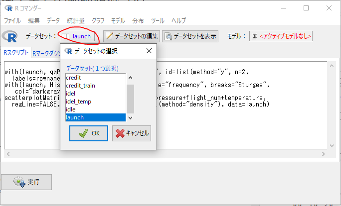
Rコマンダーでの分析

> challenger <- read_csv("challenger.csv")
> library(Rcmdr)

スクリプト

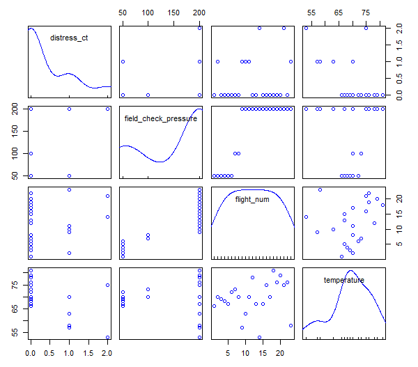
散布図行列を表示するRコマンダーのスクリプトと線形回帰モデルを作成するスクリプト。

Rcmdr>  scatterplotMatrix(~distress_ct+field_check_pressure+flight_num+temperature, regLine=FALSE, smooth=FALSE, diagonal=list(method="density"), data=launch)

Rcmdr>  RegModel.1 <- lm(distress_ct~temperature, data=launch)
Rcmdr>  summary(RegModel.1)

Call:
lm(formula = distress_ct ~ temperature, data = launch)

Residuals:
    Min      1Q  Median      3Q     Max 
-0.5608 -0.3944 -0.0854  0.1056  1.8671 

Coefficients:
            Estimate Std. Error t value Pr(>|t|)   
(Intercept)  3.69841    1.21951   3.033  0.00633 **
temperature -0.04754    0.01744  -2.725  0.01268 * 
---
Signif. codes:  0 '***' 0.001 '**' 0.01 '*' 0.05 '.' 0.1 ' ' 1

Residual standard error: 0.5774 on 21 degrees of freedom
Multiple R-squared:  0.2613,    Adjusted R-squared:  0.2261 
F-statistic: 7.426 on 1 and 21 DF,  p-value: 0.01268

GUI

1. データセットを選択する。
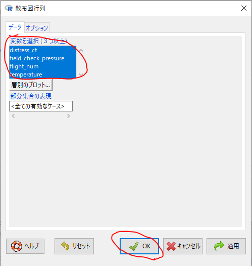
2. メニュー[グラフ]-[散布図行列…]を実行する。
3. 全ての変数を選択し、実行する。
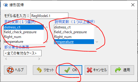
4. メニュー[統計量]-[モデルへの適合]-[線形回帰…]を実行する。
5. 目的変数としてdistress_ctを選択し、説明変数としてtemperatureを選択、実行する。

回帰木とモデル木

whitewines.csvを回帰木で分析

> install.packages("rpart")
> library(rpart)
> library(rpart.plot)
> wine <- read.csv("whitewines.csv")
> m.rpart <- rpart(quality ~., data = wine_train)
> m.rpart
n= 3750 

node), split, n, deviance, yval
      * denotes terminal node

 1) root 3750 2945.53200 5.870933  
   2) alcohol< 10.85 2372 1418.86100 5.604975  
     4) volatile.acidity>=0.2275 1611  821.30730 5.432030  
       8) volatile.acidity>=0.3025 688  278.97670 5.255814 *
       9) volatile.acidity< 0.3025 923  505.04230 5.563380 *
     5) volatile.acidity< 0.2275 761  447.36400 5.971091 *
   3) alcohol>=10.85 1378 1070.08200 6.328737  
     6) free.sulfur.dioxide< 10.5 84   95.55952 5.369048 *
     7) free.sulfur.dioxide>=10.5 1294  892.13600 6.391036  
      14) alcohol< 11.76667 629  430.11130 6.173291  
        28) volatile.acidity>=0.465 11   10.72727 4.545455 *
        29) volatile.acidity< 0.465 618  389.71680 6.202265 *
      15) alcohol>=11.76667 665  403.99400 6.596992 *
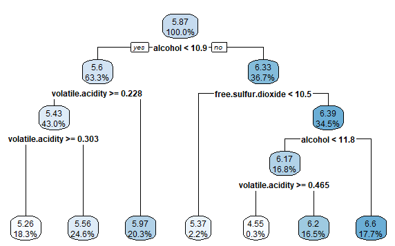
> rpart.plot(m.rpart, digits = 3)

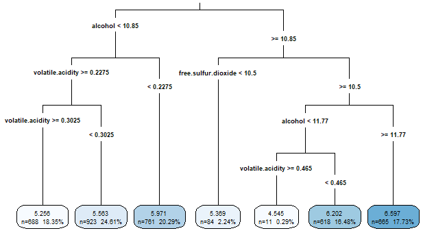
> rpart.plot(m.rpart, digits = 4, fallen.leaves = TRUE, type = 3, extra = 101)

モデル性能の評価

> p.rpart <- predict(m.rpart, wine_test)
> summary(p.rpart)
   Min. 1st Qu.  Median    Mean 3rd Qu.    Max. 
  4.545   5.563   5.971   5.893   6.202   6.597 
> summary(wine_test$quality)
   Min. 1st Qu.  Median    Mean 3rd Qu.    Max. 
  3.000   5.000   6.000   5.901   6.000   9.000 
> cor(p.rpart, wine_test$quality)
[1] 0.5369525

演習時のトラブル

*RWekaがうまくうごかない。書籍と異なる結果となる。