kerasのLSTMによる特徴量分類問題 #Keras

Qiita初投稿です。機械学習もはじめて1ヶ月のペーペーなので御手柔らかに。

今回は手始めにkerasのLSTMを用いてスマートフォンセンサー特徴量の分類問題を解きます。
取得したのは(ax,ay,az,a)と角速度(gx,gy,gz,g)です。
これらのraw dataから以下の24個の特徴量を抽出します。
Energy, Mean, Varianceの3種類を選択しました。

LSTM_classification.py

import pandas as pd
import numpy as np
import os
import seaborn as sns; sns.set()
import matplotlib.pyplot as plt

from keras.models import Sequential
from keras.layers import Activation, Dense
from keras.layers.recurrent import LSTM
from keras.layers import Dropout
from keras.preprocessing import sequence
from keras.optimizers import RMSprop

分類問題の正解ラベルは以下の8個です。
ラベルを見ればどんな行動分類をしたいかはなんとなくわかると思います。

LSTM_classification.py

calling_stopping  = pd.read_csv("completed_calling_stopping.csv", index_col = 0)
handling_stopping = pd.read_csv("completed_handling_stopping.csv", index_col = 0)
pocket_stopping   = pd.read_csv("completed_pocket_stopping.csv", index_col = 0)
swing_stopping    = pd.read_csv("completed_swing_stopping.csv", index_col = 0)
calling_walking   = pd.read_csv("completed_calling_walking.csv", index_col = 0)
handling_walking  = pd.read_csv("completed_handling_walking.csv", index_col = 0)
pocket_walking    = pd.read_csv("completed_pocket_walking.csv", index_col = 0)
swing_walking     = pd.read_csv("completed_swing_walking.csv", index_col = 0)

各ラベルに対応する整数を振ります。

LSTM_classification.py

calling_stopping["index"]  = 0
handling_stopping["index"] = 1
pocket_stopping["index"]   = 2
swing_stopping["index"]    = 3
calling_walking["index"]   = 4
handling_walking["index"]  = 5
pocket_walking["index"]    = 6
swing_walking["index"]     = 7
LABELNUM                   = 8

train_test_splitを使っても良かったんですがなんとなくマニュアルでトレーニングデータとテストデータを分けます。

LSTM_classification.py

SPLITINDEX     = 500
calling_stopping_train  = calling_stopping[:SPLITINDEX]
calling_stopping_test   = calling_stopping[SPLITINDEX + 1:]
handling_stopping_train = handling_stopping[:SPLITINDEX]
handling_stopping_test  = handling_stopping[SPLITINDEX + 1:]
pocket_stopping_train   = pocket_stopping[:SPLITINDEX]
pocket_stopping_test    = pocket_stopping[SPLITINDEX + 1:]
swing_stopping_train    = swing_stopping[:SPLITINDEX]
swing_stopping_test     = swing_stopping[SPLITINDEX + 1:]
calling_walking_train   = calling_walking[:SPLITINDEX]
calling_walking_test    = calling_walking[SPLITINDEX + 1:]
handling_walking_train  = handling_walking[:SPLITINDEX]
handling_walking_test   = handling_walking[SPLITINDEX + 1:]
pocket_walking_train    = pocket_walking[:SPLITINDEX]
pocket_walking_test     = pocket_walking[SPLITINDEX + 1:]
swing_walking_train     = swing_walking[:SPLITINDEX]
swing_walking_test      = swing_walking[SPLITINDEX + 1:]

全ラベルのデータをテスト用とトレーニング用にそれぞれくっつけます。

LSTM_classification.py

df_train = pd.concat([calling_stopping_train, handling_stopping_train, pocket_stopping_train, swing_stopping_train, calling_walking_train, handling_walking_train, pocket_walking_train, swing_walking_train])
df_test  = pd.concat([calling_stopping_test, handling_stopping_test, pocket_stopping_test, swing_stopping_test, calling_walking_test, handling_walking_test, pocket_walking_test, swing_walking_test])

テスト用とトレーニング用のデータフレームをそれぞれデータとラベルに分けます。もう少しスマートに書ける気がしますがお許しを。

LSTM_classification.py

X_train = df_train.drop('index', axis = 1)
y_train = df_train["index"]
X_test  = df_test.drop('index', axis = 1)
y_test  = df_test["index"]

後述しますがこの時のy_testを保存しておきたいので移しておきます。

LSTM_classification.py

y_test_label = y_test

このあたりが詰まったところです。kerasのLSTM関数を使う場合、トレーニングデータとテストデータの入力サイズを同じにしなければならないようです。よってテストデータのサイズをトレーニングデータのサイズに合わせるため0パディングします。

LSTM_classification.py

X_test = np.array(X_test)
zeros  = np.zeros((X_train.shape[0] - X_test.shape[0], X_train.shape[1]))
X_test = np.append(X_test, zeros, axis = 0)
X_test = pd.DataFrame(X_test)

numpyにreshapeしてデータの前処理は完了です。

LSTM_classification.py

X_train = np.reshape(X_train.values, [1, X_train.shape[0], X_train.shape[1]])
y_train = np.reshape(np.array(to_categorical(y_train)), [1, y_train.shape[0], LABELNUM])
X_test  = np.reshape(X_test.values, [1, X_test.shape[0], X_test.shape[1]])
y_test  = np.reshape(np.array(to_categorical(y_test)), [1, y_test.shape[0], LABELNUM])

ようやくモデル定義です。

LSTM_classification.py

BATCHSIZE = 32
EPOCHS    = 100
UNITNUM   = 50
optimizer = RMSprop()
model = Sequential()
model.add(LSTM(UNITNUM, input_shape = (X_train.shape[1], X_train.shape[2]), return_sequences = True))
model.add(Dropout(0.2))
model.add(Dense(LABELNUM))
model.add(Activation("softmax"))
model.compile(loss = "mean_squared_error", optimizer = optimizer, metrics = ['accuracy'])
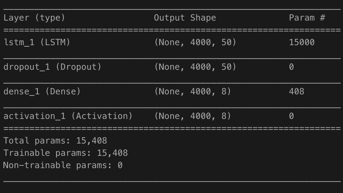
model.summary()

せっせとトレーニングします。あとで使いたいのでモデルネーム(Sequential)を引っ張ってきます。

LSTM_classification.py

history = model.fit(X_train, y_train, batch_size = BATCHSIZE, epochs = EPOCHS)
modelName = model.__class__.__name__

テストフェーズです。一旦y_predictedをcsvで出してますがもちろん出さなくても大丈夫です。

LSTM_classification.py

y_predicted = model.predict(X_test)
y_predicted = np.reshape(y_predicted, (X_train.shape[1], LABELNUM))
y_predicted = pd.DataFrame(y_predicted)
y_predicted = y_predicted.idxmax(axis = 1)
y_predicted.to_csv("predicted_%s_LSTM.csv" % modelName)

そうするともう一度numpyに戻さないといけなくて面倒ですがやります。このときさっき保存しておいたy_test_labelを使います。predeictLabelの方は0パディングしてないところまでの推定結果だけあれば良いのでそこまで引っこ抜きます。

LSTM_classification.py

trueLabel      = y_test_label.values
predictedLabel = y_predicted.values
predictedLabel = predictedLabel[:y_test.shape[1]]

大人しくconfusion matrixを出します。dpiを指定すると高画質で保存できるのでおすすめ。

LSTM_classification.py

cm = confusion_matrix(trueLabel, predictedLabel)
sns.heatmap(cm, cbar = True, cmap = 'Greens')
plt.xlabel('predictedLabel')
plt.ylabel('trueLabel');
plt.savefig("CM_%s_LSTM.png" % modelName, format = 'png', dpi = 300)

lossとaccuracyの遷移図を保存します

LSTM_classification.py

def plot_history_loss(fit):
    axL.plot(fit.history['loss'], label = "for training", color = 'dodgerblue')
    axL.set_title('model loss')
    axL.set_xlabel('epoch')
    axL.set_ylabel('loss')
def plot_history_accuracy(fit):
    axR.plot(fit.history['acc'], label = "for training", color = 'dodgerblue')
    axR.set_title('model accuracy')
    axR.set_xlabel('epoch')
    axR.set_ylabel('accuracy')

fig, (axL, axR) = plt.subplots(ncols = 2, figsize = (10,5))
plt.subplots_adjust(wspace = 0.5)
plot_history_loss(history)
plot_history_accuracy(history)
fig.savefig("loss_and_accuracy_LSTM.png", format = 'png', dpi = 300)

以上でおしまいです。model summaryは以下の通りです。

またconfusion matrixとloss and accuracyは以下の通りです。

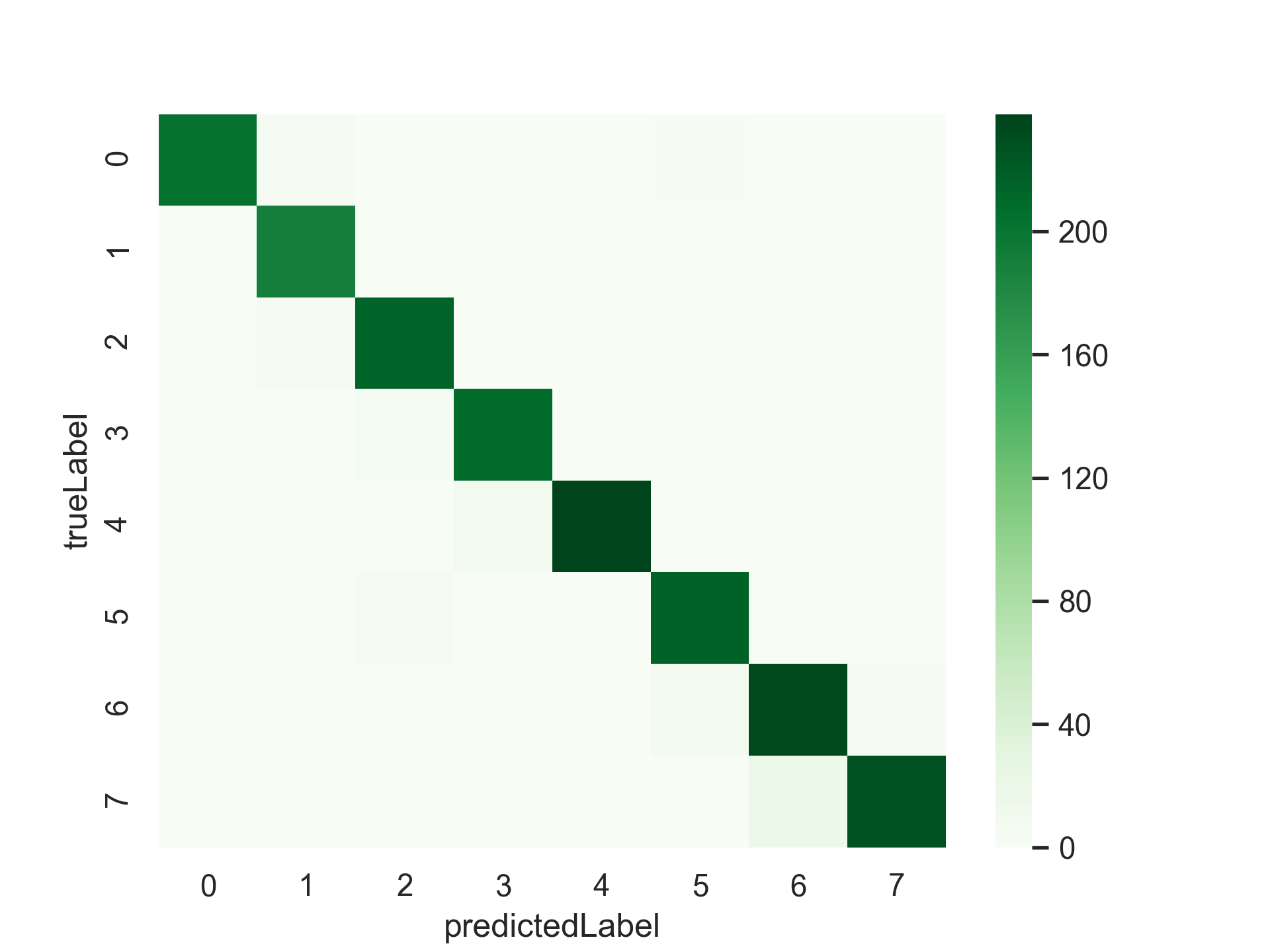
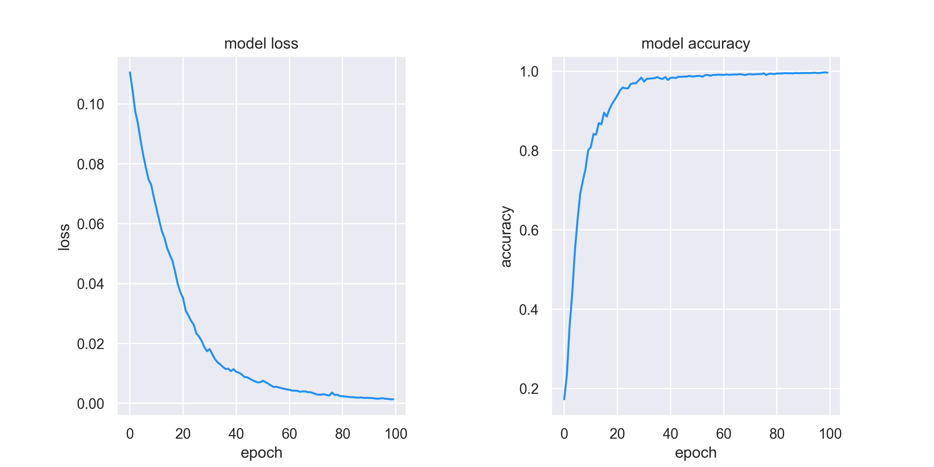
いい感じに分類できました。