ガウス過程はたいてい回帰モデルの拡張として導入されることが多いです。しかし、その場合回帰モデルのベイズ推定を理解してからでないと、ガウス過程がなんなのかよく分かりません。この記事では、とりあえずガウス過程の定義とPythonコードの例だけをガウス分布から順を追って説明します。
ガウス分布
まず、確率分布のひとつであるガウス分布の確率密度関数は、平均$\mu$と分散$\sigma^2$をパラメーターとして次のように定義されます。
$$
p(x) := \frac{1}{ \sqrt{2\pi \sigma^2} } \exp(-\frac{(x - \mu)^2}{2\sigma^2} ) \sim \mathcal{N}(\mu, \sigma^2)
$$
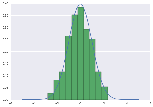
平均$\mu=0$、分散$\sigma^2 = 1$のガウス分布の確率密度関数と標本をプロットするコードは次のように書けます。
import numpy as np
import matplotlib.pyplot as plt
import seaborn
from scipy.stats import norm

# 平均
mu = 0
# 標準偏差 ( = 分散^{1/2} )
sigma = 1

x = np.linspace(-5, 5)
# 確率密度関数
p = norm.pdf(x, mu, sigma)
plt.plot(x, p)
# 標本
s = np.random.normal(mu, sigma, 500)
count, bins, ignored = plt.hist(s, normed=True)
多次元ガウス分布
次に、多次元ガウス分布の確率密度関数は$N$次元の平均ベクトルの$\mu$と$N\times N$の分散共分散行列$\Sigma$をパラメーターとして、次のように定義されます。
$$
p(x) := \frac{1}{\sqrt{ (2\pi)^n |\Sigma| }} \exp(-\frac{1}{2} (x-\mu)^T \Sigma^{-1} (x-\mu)) \sim \mathcal{N}(\mu,\Sigma)
$$
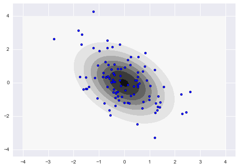
平均$\mu = (0, 0)$、分散共分散行列
\Sigma = \begin{pmatrix} 1& -0.5\\ -0.5 & 1.5\end{pmatrix}
の2次元ガウス分布の確率密度関数と標本をプロットするコードは次のように書けます。scipy、numpyを使えば関数を呼ぶだけです。
from scipy.stats import multivariate_normal

# 2次元のメッシュの座標とその座標での値をしまう3次元の変数を用意
N = 60
X = np.linspace(-4, 4, N)
Y = np.linspace(-4, 4, N)
X, Y = np.meshgrid(X, Y)
pos = np.empty(X.shape + (2,))
pos[:, :, 0] = X
pos[:, :, 1] = Y

# 平均
mu_multi = np.array([0., 0.])
#  分散共分散行列
Sigma_multi = np.array([[ 1. , -0.5], [-0.5,  1.5]])

# 確率密度関数
F = multivariate_normal(mu_multi, Sigma_multi)
p_multi = F.pdf(pos)
cset = plt.contourf(X, Y, p_multi )

# 標本
s_multi = np.random.multivariate_normal(mu_multi, Sigma_multi, 100)
plt.scatter(s_multi[:,0], s_multi[:,1])
ガウス過程
ガウス過程は、無限次元のガウス分布と考えることができます。
任意の時刻の集合$t = (t_1, t_2, \cdots, t_k)$に対して、関数$f(t)$が平均$\mu=m(t)$、分散共分散行列$\Sigma = K(t,t)$の$k$次元ガウス分布に従うとき、すなわち、$f(t) \sim N( m(t), K(t,t) )$となるとき、$f(t)$をガウス過程と呼びます。また、分散共分散行列の要素$k(t_i, t_j) = (K(t,t))_{ij}$をカーネル関数と呼びます。
平均を0ベクトル、
$$
m(t) = (0, \cdots, 0)
$$
カーネル関数をパラメーター$\sigma, l$をもつ
$$
k(t_i, t_j) = \sigma^2 \exp (-\frac{1}{2l^2} (t_i-t_j)^2)
$$
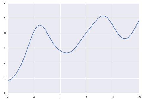
としたときの(このカーネル関数はsquared exponential カーネルと呼ばれます)、ガウス過程のサンプル経路をプロットするコードは次のようになります。
ここでポイントは、カーネル関数が時刻の距離についての指数関数になっているので、定性的には微小時間離れた2点の相関係数はほぼ1になり、このカーネル関数を使ったガウス過程はなめらかになります。
t = np.linspace(0, 10)
t = np.reshape(t, (1,t.size))

# カーネル関数を成分にもつ行列
def K(t):
    sigma = 1
    l = 1
    rows = np.repeat(t, t.size, axis=0)
    cols = np.repeat(t.T, t.size, axis=1)
    mat = cols-rows
    return sigma**2  * np.exp(- np.multiply(mat , mat) / (2 * l **2))

Sigma = K(t)
mu = np.zeros(t.size)
s_gp = np.random.multivariate_normal(mu, Sigma)
plt.plot(t[0,:], s_gp)