【ラビットチャレンジ】 機械学習 第3章 ロジスティック回帰モデル

ロジスティック回帰モデル

• 分類問題（クラス分類）
  • ある入力をクラスに分類する
  • 入力（各要素を説明変数または特徴量と呼ぶ）
    • $m$次元のベクトル
  • 出力（目的変数）
    • $0$ or $1$ の値
• ロジスティック線形回帰モデル
  • 入力と$m$次元のパラメータの線形結合をシグモイド関数に入力する
  • 出力は$y = 1$となる確率の値となる．
    • 確率が設定した閾値を超えたときTrueとする．

シグモイド関数

• シグモイド関数の性質

  • 入力は実数，出力は$0$~$1$の値．
  • 単調増加関数． $$\sigma(x) = \frac{1}{1+\exp(-ax)}$$
  • シグモイド関数の微分は，シグモイド関数自身で表現できる． $$\frac{\partial\sigma(x)}{\partial x}=a\sigma(x)(1-\sigma(x))$$
    • この性質により，尤度関数の微分を行う際に計算が容易．

• シグモイド関数の出力を$Y=1$になる確率に対応させる．
  $$P(Y=1|x)=\sigma(w_0+w_1x_1+\cdots +w_mx_m)$$

最尤推定

• 尤度関数
  • 確率分布を仮定し，観測されたデータから，その確率分布が尤もらしいかを表現したもの．
• 最尤推定
  • 尤度関数を最大化するようなパラメータを選ぶ推定方法．
    • 尤度関数の対数をとるのがセオリー．

勾配降下法(Gradient descent)

• 反復学習によりパラメータを逐次的に更新する．
• 最尤法は解析的に解けないのでパラメータを逐次更新することで最大値を求める．
  • パラメータを更新するのに全データに対する和を求める必要があるが，必要メモリや計算量が大きくなるので大変．⇛確率的勾配降下法(SGD)を利用して解決する．
    • データをランダムに選び，１つのデータでパラメータを１回更新する．

混同行列(Confusion Matrix)

• 予測結果が正解
  • True Positive / True Negative

• 予測結果が不正解

  • False Positive / False Negative

• 分類の評価方法

  • 正解率 $$\frac{TP+TN}{TP+FN+FP+TN}$$
  • 再現率(Recall)
    • 見逃しが多くてもより正確な予測をしたい $$\frac{TP}{TP+FN}$$
  • 適合率(Precision)
    • 誤りが多くても抜け漏れは少ない予測をしたい $$\frac{TP}{TP+FP}$$
  • F値
    • 再現率と適合率はトレードオフだが，どちらも高いモデルが理想的．
      • RecallとPrecisionの調和平均を取る．

ハンズオン

0. データ表示

skl_logistic_regression.ipynb

#from モジュール名 import クラス名（もしくは関数名や変数名）
import pandas as pd
from pandas import DataFrame
import numpy as np
import matplotlib.pyplot as plt
import seaborn as sns

#matplotlibをinlineで表示するためのおまじない (plt.show()しなくていい)
%matplotlib inline

skl_logistic_regression.ipynb

# titanic data csvファイルの読み込み
titanic_df = pd.read_csv('../data/titanic_train.csv')

skl_logistic_regression.ipynb

# ファイルの先頭部を表示し、データセットを確認する
titanic_df.head(5)

	PassengerId	Survived	Pclass	Name	Sex	Age	SibSp	Parch	Ticket	Fare	Cabin	Embarked
0	1	0	3	Braund, Mr. Owen Harris	male	22.0	1	0	A/5 21171	7.2500	NaN	S
1	2	1	1	Cumings, Mrs. John Bradley (Florence Briggs Th...	female	38.0	1	0	PC 17599	71.2833	C85	C
2	3	1	3	Heikkinen, Miss. Laina	female	26.0	0	0	STON/O2. 3101282	7.9250	NaN	S
3	4	1	1	Futrelle, Mrs. Jacques Heath (Lily May Peel)	female	35.0	1	0	113803	53.1000	C123	S
4	5	0	3	Allen, Mr. William Henry	male	35.0	0	0	373450	8.0500	NaN	S

1. ロジスティック回帰

不要なデータの削除・欠損値の補完

skl_logistic_regression.ipynb

#予測に不要と考えるからうをドロップ (本当はここの情報もしっかり使うべきだと思っています)
titanic_df.drop(['PassengerId', 'Name', 'Ticket', 'Cabin'], axis=1, inplace=True)

#一部カラムをドロップしたデータを表示
titanic_df.head()

	Survived	Pclass	Sex	Age	SibSp	Parch	Fare	Embarked
0	0	3	male	22.0	1	0	7.2500	S
1	1	1	female	38.0	1	0	71.2833	C
2	1	3	female	26.0	0	0	7.9250	S
3	1	1	female	35.0	1	0	53.1000	S
4	0	3	male	35.0	0	0	8.0500	S

skl_logistic_regression.ipynb

#nullを含んでいる行を表示
titanic_df[titanic_df.isnull().any(1)].head(10)

	Survived	Pclass	Sex	Age	SibSp	Parch	Fare	Embarked
5	0	3	male	NaN	0	0	8.4583	Q
17	1	2	male	NaN	0	0	13.0000	S
19	1	3	female	NaN	0	0	7.2250	C
26	0	3	male	NaN	0	0	7.2250	C
28	1	3	female	NaN	0	0	7.8792	Q
29	0	3	male	NaN	0	0	7.8958	S
31	1	1	female	NaN	1	0	146.5208	C
32	1	3	female	NaN	0	0	7.7500	Q
36	1	3	male	NaN	0	0	7.2292	C
42	0	3	male	NaN	0	0	7.8958	C

skl_logistic_regression.ipynb

#Ageカラムのnullを中央値で補完

#AgeFillのカラムを作る
titanic_df['AgeFill'] = titanic_df['Age'].fillna(titanic_df['Age'].mean())

#再度nullを含んでいる行を表示 (Ageのnullは補完されている)
titanic_df[titanic_df.isnull().any(1)]

#titanic_df.dtypes

	Survived	Pclass	Sex	Age	SibSp	Parch	Fare	Embarked	AgeFill
5	0	3	male	NaN	0	0	8.4583	Q	29.699118
17	1	2	male	NaN	0	0	13.0000	S	29.699118
19	1	3	female	NaN	0	0	7.2250	C	29.699118
26	0	3	male	NaN	0	0	7.2250	C	29.699118
28	1	3	female	NaN	0	0	7.8792	Q	29.699118
29	0	3	male	NaN	0	0	7.8958	S	29.699118
31	1	1	female	NaN	1	0	146.5208	C	29.699118
32	1	3	female	NaN	0	0	7.7500	Q	29.699118
36	1	3	male	NaN	0	0	7.2292	C	29.699118
42	0	3	male	NaN	0	0	7.8958	C	29.699118
45	0	3	male	NaN	0	0	8.0500	S	29.699118
46	0	3	male	NaN	1	0	15.5000	Q	29.699118
47	1	3	female	NaN	0	0	7.7500	Q	29.699118
48	0	3	male	NaN	2	0	21.6792	C	29.699118
55	1	1	male	NaN	0	0	35.5000	S	29.699118
61	1	1	female	38.0	0	0	80.0000	NaN	38.000000
64	0	1	male	NaN	0	0	27.7208	C	29.699118
65	1	3	male	NaN	1	1	15.2458	C	29.699118
76	0	3	male	NaN	0	0	7.8958	S	29.699118
77	0	3	male	NaN	0	0	8.0500	S	29.699118
82	1	3	female	NaN	0	0	7.7875	Q	29.699118
87	0	3	male	NaN	0	0	8.0500	S	29.699118
95	0	3	male	NaN	0	0	8.0500	S	29.699118
101	0	3	male	NaN	0	0	7.8958	S	29.699118
107	1	3	male	NaN	0	0	7.7750	S	29.699118
109	1	3	female	NaN	1	0	24.1500	Q	29.699118
121	0	3	male	NaN	0	0	8.0500	S	29.699118
126	0	3	male	NaN	0	0	7.7500	Q	29.699118
128	1	3	female	NaN	1	1	22.3583	C	29.699118
140	0	3	female	NaN	0	2	15.2458	C	29.699118
...	...	...	...	...	...	...	...	...	...
727	1	3	female	NaN	0	0	7.7375	Q	29.699118
732	0	2	male	NaN	0	0	0.0000	S	29.699118
738	0	3	male	NaN	0	0	7.8958	S	29.699118
739	0	3	male	NaN	0	0	7.8958	S	29.699118
740	1	1	male	NaN	0	0	30.0000	S	29.699118
760	0	3	male	NaN	0	0	14.5000	S	29.699118
766	0	1	male	NaN	0	0	39.6000	C	29.699118
768	0	3	male	NaN	1	0	24.1500	Q	29.699118
773	0	3	male	NaN	0	0	7.2250	C	29.699118
776	0	3	male	NaN	0	0	7.7500	Q	29.699118
778	0	3	male	NaN	0	0	7.7375	Q	29.699118
783	0	3	male	NaN	1	2	23.4500	S	29.699118
790	0	3	male	NaN	0	0	7.7500	Q	29.699118
792	0	3	female	NaN	8	2	69.5500	S	29.699118
793	0	1	male	NaN	0	0	30.6958	C	29.699118
815	0	1	male	NaN	0	0	0.0000	S	29.699118
825	0	3	male	NaN	0	0	6.9500	Q	29.699118
826	0	3	male	NaN	0	0	56.4958	S	29.699118
828	1	3	male	NaN	0	0	7.7500	Q	29.699118
829	1	1	female	62.0	0	0	80.0000	NaN	62.000000
832	0	3	male	NaN	0	0	7.2292	C	29.699118
837	0	3	male	NaN	0	0	8.0500	S	29.699118
839	1	1	male	NaN	0	0	29.7000	C	29.699118
846	0	3	male	NaN	8	2	69.5500	S	29.699118
849	1	1	female	NaN	1	0	89.1042	C	29.699118
859	0	3	male	NaN	0	0	7.2292	C	29.699118
863	0	3	female	NaN	8	2	69.5500	S	29.699118
868	0	3	male	NaN	0	0	9.5000	S	29.699118
878	0	3	male	NaN	0	0	7.8958	S	29.699118
888	0	3	female	NaN	1	2	23.4500	S	29.699118

179 rows × 9 columns

1. ロジスティック回帰

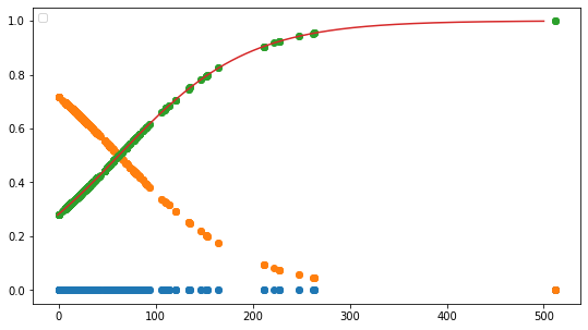
実装(チケット価格から生死を判別)

skl_logistic_regression.ipynb

#運賃だけのリストを作成
data1 = titanic_df.loc[:, ["Fare"]].values

skl_logistic_regression.ipynb

#生死フラグのみのリストを作成
label1 =  titanic_df.loc[:,["Survived"]].values

skl_logistic_regression.ipynb

from sklearn.linear_model import LogisticRegression

skl_logistic_regression.ipynb

#ロジスティック回帰
model=LogisticRegression()

skl_logistic_regression.ipynb

label=np.reshape(label1,(-1))
model.fit(data1, label)

/Users/***/anaconda3/lib/python3.7/site-packages/sklearn/linear_model/logistic.py:432: FutureWarning: Default solver will be changed to 'lbfgs' in 0.22. Specify a solver to silence this warning.
  FutureWarning)





LogisticRegression(C=1.0, class_weight=None, dual=False, fit_intercept=True,
                   intercept_scaling=1, l1_ratio=None, max_iter=100,
                   multi_class='warn', n_jobs=None, penalty='l2',
                   random_state=None, solver='warn', tol=0.0001, verbose=0,
                   warm_start=False)

skl_logistic_regression.ipynb

#運賃をドルで入れてみる．62ドル以上で生き残る予想．
model.predict([[62]])

array([1])

skl_logistic_regression.ipynb

#確率の表示．[死亡, 生存]．62ドルで生存の確率が50%を超えるので，predictで生存を返す．
model.predict_proba([[62]])

array([[0.49968899, 0.50031101]])

skl_logistic_regression.ipynb

X_test_value = model.decision_function(data1) 

skl_logistic_regression.ipynb

# # 決定関数値（絶対値が大きいほど識別境界から離れている）
# X_test_value = model.decision_function(X_test) 
# # 決定関数値をシグモイド関数で確率に変換
# X_test_prob = normal_sigmoid(X_test_value) 

skl_logistic_regression.ipynb

print (model.intercept_)

print (model.coef_)

[-0.93290045]
[[0.01506685]]

skl_logistic_regression.ipynb

w_0 = model.intercept_[0]
w_1 = model.coef_[0,0]

# def normal_sigmoid(x):
#     return 1 / (1+np.exp(-x))

def sigmoid(x):
    return 1 / (1+np.exp(-(w_1*x+w_0)))

x_range = np.linspace(-1, 500, 3000)

plt.figure(figsize=(9,5))
#plt.xkcd()
plt.legend(loc=2)


# plt.ylim(-0.1, 1.1)
# plt.xlim(-10, 10)

# plt.plot([-10,10],[0,0], "k", lw=1)
# plt.plot([0,0],[-1,1.5], "k", lw=1)
plt.plot(data1,np.zeros(len(data1)), 'o')
plt.plot(data1, model.predict_proba(data1), 'o')
plt.plot(x_range, sigmoid(x_range), '-')
#plt.plot(x_range, normal_sigmoid(x_range), '-')

No handles with labels found to put in legend.





[<matplotlib.lines.Line2D at 0x1a2546bc88>]

1. ロジスティック回帰

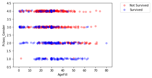
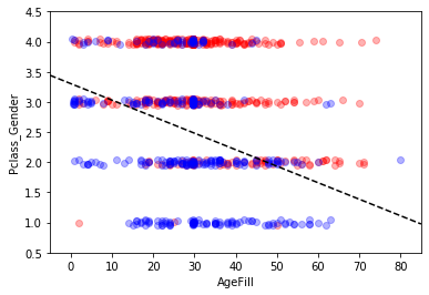
実装(2変数から生死を判別)

skl_logistic_regression.ipynb

#AgeFillの欠損値を埋めたので
#titanic_df = titanic_df.drop(['Age'], axis=1)

skl_logistic_regression.ipynb

#Genderカラムに性別を1/0に変換したものを入れる．
titanic_df['Gender'] = titanic_df['Sex'].map({'female': 0, 'male': 1}).astype(int)

skl_logistic_regression.ipynb

titanic_df.head()

	Survived	Pclass	Sex	Age	SibSp	Parch	Fare	Embarked	AgeFill	Gender
0	0	3	male	22.0	1	0	7.2500	S	22.0	1
1	1	1	female	38.0	1	0	71.2833	C	38.0	0
2	1	3	female	26.0	0	0	7.9250	S	26.0	0
3	1	1	female	35.0	1	0	53.1000	S	35.0	0
4	0	3	male	35.0	0	0	8.0500	S	35.0	1

skl_logistic_regression.ipynb

#生存率が高い=地位が高い(Pclassが小さい)，性別が女性(0)という仮説から新たな変数を作る
titanic_df['Pclass_Gender'] = titanic_df['Pclass'] + titanic_df['Gender']

skl_logistic_regression.ipynb

titanic_df.head()

	Survived	Pclass	Sex	Age	SibSp	Parch	Fare	Embarked	AgeFill	Gender	Pclass_Gender
0	0	3	male	22.0	1	0	7.2500	S	22.0	1	4
1	1	1	female	38.0	1	0	71.2833	C	38.0	0	1
2	1	3	female	26.0	0	0	7.9250	S	26.0	0	3
3	1	1	female	35.0	1	0	53.1000	S	35.0	0	1
4	0	3	male	35.0	0	0	8.0500	S	35.0	1	4

skl_logistic_regression.ipynb

#いらないカラムをドロップする
titanic_df = titanic_df.drop(['Pclass', 'Sex', 'Gender','Age'], axis=1)

skl_logistic_regression.ipynb

titanic_df.head()

	Survived	SibSp	Parch	Fare	Embarked	AgeFill	Pclass_Gender
0	0	1	0	7.2500	S	22.0	4
1	1	1	0	71.2833	C	38.0	1
2	1	0	0	7.9250	S	26.0	3
3	1	1	0	53.1000	S	35.0	1
4	0	0	0	8.0500	S	35.0	4

skl_logistic_regression.ipynb

# 重要だよ！！！
# 境界線の式
#   w_1・x + w_2・y + w_0 = 0
#   ⇒ y = (-w_1・x - w_0) / w_2

# # 境界線 プロット
# plt.plot([-2,2], map(lambda x: (-w_1 * x - w_0)/w_2, [-2,2]))

# # データを重ねる
# plt.scatter(X_train_std[y_train==0, 0], X_train_std[y_train==0, 1], c='red', marker='x', label='train 0')
# plt.scatter(X_train_std[y_train==1, 0], X_train_std[y_train==1, 1], c='blue', marker='x', label='train 1')
# plt.scatter(X_test_std[y_test==0, 0], X_test_std[y_test==0, 1], c='red', marker='o', s=60, label='test 0')
# plt.scatter(X_test_std[y_test==1, 0], X_test_std[y_test==1, 1], c='blue', marker='o', s=60, label='test 1')

skl_logistic_regression.ipynb

np.random.seed = 0

xmin, xmax = -5, 85
ymin, ymax = 0.5, 4.5

index_survived = titanic_df[titanic_df["Survived"]==0].index
index_notsurvived = titanic_df[titanic_df["Survived"]==1].index

from matplotlib.colors import ListedColormap
fig, ax = plt.subplots()
cm = plt.cm.RdBu
cm_bright = ListedColormap(['#FF0000', '#0000FF'])
sc = ax.scatter(titanic_df.loc[index_survived, 'AgeFill'],
                titanic_df.loc[index_survived, 'Pclass_Gender']+(np.random.rand(len(index_survived))-0.5)*0.1,
                color='r', label='Not Survived', alpha=0.3)
sc = ax.scatter(titanic_df.loc[index_notsurvived, 'AgeFill'],
                titanic_df.loc[index_notsurvived, 'Pclass_Gender']+(np.random.rand(len(index_notsurvived))-0.5)*0.1,
                color='b', label='Survived', alpha=0.3)
ax.set_xlabel('AgeFill')
ax.set_ylabel('Pclass_Gender')
ax.set_xlim(xmin, xmax)
ax.set_ylim(ymin, ymax)
ax.legend(bbox_to_anchor=(1.4, 1.03))

<matplotlib.legend.Legend at 0x1a245c0be0>

skl_logistic_regression.ipynb

#運賃だけのリストを作成
data2 = titanic_df.loc[:, ["AgeFill", "Pclass_Gender"]].values

skl_logistic_regression.ipynb

data2

array([[22.        ,  4.        ],
       [38.        ,  1.        ],
       [26.        ,  3.        ],
       ...,
       [29.69911765,  3.        ],
       [26.        ,  2.        ],
       [32.        ,  4.        ]])

skl_logistic_regression.ipynb

#生死フラグのみのリストを作成
label2 =  titanic_df.loc[:,["Survived"]].values

skl_logistic_regression.ipynb

model2 = LogisticRegression()

skl_logistic_regression.ipynb

label=np.reshape(label2,(-1))
model2.fit(data2, label)

/Users/***/anaconda3/lib/python3.7/site-packages/sklearn/linear_model/logistic.py:432: FutureWarning: Default solver will be changed to 'lbfgs' in 0.22. Specify a solver to silence this warning.
  FutureWarning)





LogisticRegression(C=1.0, class_weight=None, dual=False, fit_intercept=True,
                   intercept_scaling=1, l1_ratio=None, max_iter=100,
                   multi_class='warn', n_jobs=None, penalty='l2',
                   random_state=None, solver='warn', tol=0.0001, verbose=0,
                   warm_start=False)

skl_logistic_regression.ipynb

model2.predict([[10,1]])

array([1])

skl_logistic_regression.ipynb

model2.predict_proba([[10,1]])

array([[0.06072391, 0.93927609]])

skl_logistic_regression.ipynb

titanic_df.head(3)

	Survived	SibSp	Parch	Fare	Embarked	AgeFill	Pclass_Gender
0	0	1	0	7.2500	S	22.0	4
1	1	1	0	71.2833	C	38.0	1
2	1	0	0	7.9250	S	26.0	3

skl_logistic_regression.ipynb

h = 0.02
xmin, xmax = -5, 85
ymin, ymax = 0.5, 4.5
xx, yy = np.meshgrid(np.arange(xmin, xmax, h), np.arange(ymin, ymax, h))
Z = model2.predict_proba(np.c_[xx.ravel(), yy.ravel()])[:, 1]
Z = Z.reshape(xx.shape)

fig, ax = plt.subplots()
levels = np.linspace(0, 1.0)
cm = plt.cm.RdBu
cm_bright = ListedColormap(['#FF0000', '#0000FF'])
#contour = ax.contourf(xx, yy, Z, cmap=cm, levels=levels, alpha=0.5)

sc = ax.scatter(titanic_df.loc[index_survived, 'AgeFill'],
                titanic_df.loc[index_survived, 'Pclass_Gender']+(np.random.rand(len(index_survived))-0.5)*0.1,
                color='r', label='Not Survived', alpha=0.3)
sc = ax.scatter(titanic_df.loc[index_notsurvived, 'AgeFill'],
                titanic_df.loc[index_notsurvived, 'Pclass_Gender']+(np.random.rand(len(index_notsurvived))-0.5)*0.1,
                color='b', label='Survived', alpha=0.3)

ax.set_xlabel('AgeFill')
ax.set_ylabel('Pclass_Gender')
ax.set_xlim(xmin, xmax)
ax.set_ylim(ymin, ymax)
#fig.colorbar(contour)

x1 = xmin
x2 = xmax
y1 = -1*(model2.intercept_[0]+model2.coef_[0][0]*xmin)/model2.coef_[0][1]
y2 = -1*(model2.intercept_[0]+model2.coef_[0][0]*xmax)/model2.coef_[0][1]
ax.plot([x1, x2] ,[y1, y2], 'k--')

[<matplotlib.lines.Line2D at 0x1a251be5f8>]

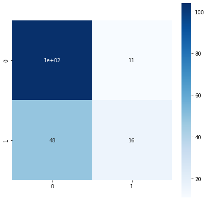
2. モデル評価

混同行列とクロスバリデーション

skl_logistic_regression.ipynb

from sklearn.model_selection import train_test_split

skl_logistic_regression.ipynb

#学習用のデータとテスト用のデータに分ける
traindata1, testdata1, trainlabel1, testlabel1 = train_test_split(data1, label1, test_size=0.2)
traindata1.shape
trainlabel1.shape

(712, 1)

skl_logistic_regression.ipynb

traindata2, testdata2, trainlabel2, testlabel2 = train_test_split(data2, label2, test_size=0.2)
traindata2.shape
trainlabel2.shape
#本来は同じデータセットを分割しなければいけない。(簡易的に別々に分割している。)

(712, 1)

skl_logistic_regression.ipynb

data = titanic_df.loc[:, ].values
label =  titanic_df.loc[:,["Survived"]].values
traindata, testdata, trainlabel, testlabel = train_test_split(data, label, test_size=0.2)
traindata.shape
trainlabel.shape

(712, 1)

skl_logistic_regression.ipynb

eval_model1=LogisticRegression()
eval_model2=LogisticRegression()
#eval_model=LogisticRegression()

skl_logistic_regression.ipynb

trainlabel01=np.reshape(trainlabel1,(-1))
trainlabel02=np.reshape(trainlabel2,(-1))
predictor_eval1=eval_model1.fit(traindata1, trainlabel01).predict(testdata1)
predictor_eval2=eval_model2.fit(traindata2, trainlabel02).predict(testdata2)
#predictor_eval=eval_model.fit(traindata, trainlabel).predict(testdata)

/Users/***/anaconda3/lib/python3.7/site-packages/sklearn/linear_model/logistic.py:432: FutureWarning: Default solver will be changed to 'lbfgs' in 0.22. Specify a solver to silence this warning.
  FutureWarning)
/Users/***/anaconda3/lib/python3.7/site-packages/sklearn/linear_model/logistic.py:432: FutureWarning: Default solver will be changed to 'lbfgs' in 0.22. Specify a solver to silence this warning.
  FutureWarning)

skl_logistic_regression.ipynb

eval_model1.score(traindata1, trainlabel1)

0.6615168539325843

skl_logistic_regression.ipynb

eval_model1.score(testdata1,testlabel1)

0.6703910614525139

skl_logistic_regression.ipynb

eval_model2.score(traindata2, trainlabel2)

0.7752808988764045

skl_logistic_regression.ipynb

eval_model2.score(testdata2,testlabel2)

0.8044692737430168

skl_logistic_regression.ipynb

from sklearn import metrics
print(metrics.classification_report(testlabel1, predictor_eval1))
print(metrics.classification_report(testlabel2, predictor_eval2))

              precision    recall  f1-score   support

           0       0.68      0.90      0.78       115
           1       0.59      0.25      0.35        64

    accuracy                           0.67       179
   macro avg       0.64      0.58      0.57       179
weighted avg       0.65      0.67      0.63       179

              precision    recall  f1-score   support

           0       0.82      0.88      0.85       112
           1       0.78      0.67      0.72        67

    accuracy                           0.80       179
   macro avg       0.80      0.78      0.78       179
weighted avg       0.80      0.80      0.80       179

skl_logistic_regression.ipynb

from sklearn.metrics import confusion_matrix
confusion_matrix1=confusion_matrix(testlabel1, predictor_eval1)
confusion_matrix2=confusion_matrix(testlabel2, predictor_eval2)

skl_logistic_regression.ipynb

confusion_matrix1

array([[104,  11],
       [ 48,  16]])

skl_logistic_regression.ipynb

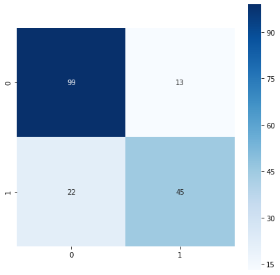
confusion_matrix2

array([[99, 13],
       [22, 45]])

skl_logistic_regression.ipynb

fig = plt.figure(figsize = (7,7))
#plt.title(title)
sns.heatmap(
    confusion_matrix1,
    vmin=None,
    vmax=None,
    cmap="Blues",
    center=None,
    robust=False,
    annot=True, fmt='.2g',
    annot_kws=None,
    linewidths=0,
    linecolor='white',
    cbar=True,
    cbar_kws=None,
    cbar_ax=None,
    square=True, ax=None, 
    #xticklabels=columns,
    #yticklabels=columns,
    mask=None)

<matplotlib.axes._subplots.AxesSubplot at 0x1112c34a8>

skl_logistic_regression.ipynb

fig = plt.figure(figsize = (7,7))
#plt.title(title)
sns.heatmap(
    confusion_matrix2,
    vmin=None,
    vmax=None,
    cmap="Blues",
    center=None,
    robust=False,
    annot=True, fmt='.2g',
    annot_kws=None,
    linewidths=0,
    linecolor='white',
    cbar=True,
    cbar_kws=None,
    cbar_ax=None,
    square=True, ax=None, 
    #xticklabels=columns,
    #yticklabels=columns,
    mask=None)

<matplotlib.axes._subplots.AxesSubplot at 0x1a28e5aa90>

skl_logistic_regression.ipynb

#Paired categorical plots

import seaborn as sns
sns.set(style="whitegrid")

# Load the example Titanic dataset
titanic = sns.load_dataset("titanic")

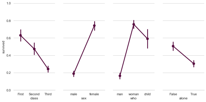
# Set up a grid to plot survival probability against several variables
g = sns.PairGrid(titanic, y_vars="survived",
                 x_vars=["class", "sex", "who", "alone"],
                 height=5, aspect=.5)

# Draw a seaborn pointplot onto each Axes
g.map(sns.pointplot, color=sns.xkcd_rgb["plum"])
g.set(ylim=(0, 1))
sns.despine(fig=g.fig, left=True)

plt.show()

skl_logistic_regression.ipynb

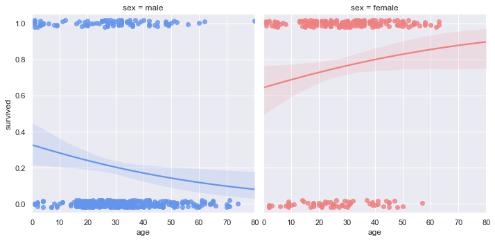
#Faceted logistic regression

import seaborn as sns
sns.set(style="darkgrid")

# Load the example titanic dataset
df = sns.load_dataset("titanic")

# Make a custom palette with gendered colors
pal = dict(male="#6495ED", female="#F08080")

# Show the survival proability as a function of age and sex
g = sns.lmplot(x="age", y="survived", col="sex", hue="sex", data=df,
               palette=pal, y_jitter=.02, logistic=True)
g.set(xlim=(0, 80), ylim=(-.05, 1.05))
plt.show()

考察

• 適宜Warningを修正．
• 多くの項目からPclassとGenderを選び，さらにそれらを合算してPclass-Genderという１つの項目を作成して検証しているが，それを行う根拠があるのか，テクニックの１つなのか，不明であった．
• ただし，項目を統合すると１つ次元を減らせるので，グラフ化しやすく視覚的に理解しやすくなる．
  • 資料の作り方，見せ方も重要．項目を統合する根拠も必要．

DeepLearning ラビットチャレンジ