回帰問題
- ある入力から出力を予測する問題.
- 直線で予測 → 線形回帰
- 曲線で予測 → 非線形回帰
回帰で扱うデータ
- 入力(各要素を説明変数または特徴量と呼ぶ)
- m次元のベクトル $$ \boldsymbol{x} = (x_1, x_2, \cdots, x_m)^T \in \mathbb{R}^m$$
- 出力(目的変数)
- スカラー値 $$ y \in \mathbb{R}^1$$
線形回帰モデル
- 回帰問題を解くための機械学習モデルの一つ
- m次元の入力とm次元のパラメータの線形結合を出力するモデル
- 慣例として予測値にはハットをつける
線形結合(入力とパラメータの内積)
パラメータを $$ \boldsymbol{w} = (w_1, w_2, \cdots, w_m)^T \in \mathbb{R}^m$$ とすると,
予測値 $\hat{y}$ は,$$ \hat{y} = \boldsymbol{w}^T \boldsymbol{x} + w_0 = \sum_{j=1}^{m}w_jx_j+w_0$$と書ける.
$w_0$ は切片であり $x_0 = 1$ とおくと,$$ \hat{y} = \sum_{j=0}^{m}w_jx_j$$と書ける.
モデルのパラメータ
- モデルに含まれる推定すべき未知のパラメータ
- 特徴量が予測値に対してどのように影響を与えるかを決定する重みの集合.
パラメータを推定する
データセット(x, y)によるパラメータwに関する連立方程式の行列表現
説明変数の集合$\{\boldsymbol{x}_1, \cdots, \boldsymbol{x}_n \}$と,それらに対応する目的変数の集合 $\{y_1, \cdots, y_n \}$ が与えられているとき,それらに対応する誤差の集合を $\{\epsilon_1, \cdots, \epsilon_n \}$ とすると,線形回帰モデルは以下のように表される.線形回帰モデルは以下のように表される.$$\boldsymbol{y} = \boldsymbol{Xw} + \boldsymbol{\epsilon}$$
ただし, $$X=(\boldsymbol{x}_1, \cdots, \boldsymbol{x}_n)^T$$ $$\boldsymbol{x}_i = (1, x_{i1}, \cdots, x_{im})^T$$ $$\boldsymbol{\epsilon} = (\epsilon_1, \cdots, \epsilon_n)^T$$ $$\boldsymbol{w} = ( w_0, \cdots, w_m)^T$$
データの分割とモデルの汎化性能測定
- データの分割
-
学習用データ:機械学習モデルの学習に利用するデータ
$$\{(\boldsymbol{x}_i^{(train)}, y^{(train)}); i=1,\cdots,n_{train}\}$$ -
検証用データ:学習済みモデルの性能を検証するためのデータ
$$\{(\boldsymbol{x}_i^{(test)}, y^{(test)}); i=1,\cdots,n_{test}\}$$
-
- なぜ分割するか
- モデルの汎化性能を測るため.
- 与えられたデータへの当てはまりの良さではなく,未知のデータに対してどれくらい精度が高いかを測りたい.
学習用データを利用して推定パラメータを学習し,検証用データを用いて汎化性能を検証する.
最小二乗法
-
学習誤差
$$MSE_{train} = \frac{1}{n_{train}}\sum_{i=1}^{n_{train}}(\hat{y}_i^{(train)}-y_i^{(train)})^2$$ -
検証誤差
$$MSE_{test} = \frac{1}{n_{test}}\sum_{i=1}^{n_{test}}(\hat{y}_i^{(test)}-y_i^{(test)})^2$$ -
学習誤差を最小二乗法で解く
- 学習データの平均二乗誤差を最小とするパラメータを探索する.
- 学習データの平均二乗誤差の最小化は,その勾配が0になる点を求めれば良い.(数学的に陽に解ける)
\begin{align}
&\frac{\partial}{\partial\boldsymbol{w}}MSE_{train}=0\\

\Leftrightarrow
&\frac{\partial}{\partial\boldsymbol{w}}
\Bigl[
\frac{1}{n_{train}}\sum_{i=1}^{n_{train}}(\hat{y}\_i^{(train)}-y\_i^{(train)})^2
\Bigr] = 0\\

\Leftrightarrow
&\frac{1}{n_{train}}\frac{\partial}{\partial\boldsymbol{w}}
\Bigl[
(\boldsymbol{X}^{(train)}\boldsymbol{w}-\boldsymbol{y}^{(train)})^T
(\boldsymbol{X}^{(train)}\boldsymbol{w}-\boldsymbol{y}^{(train)})
\Bigr] = 0\\

\Leftrightarrow
&\frac{1}{n_{train}}\frac{\partial}{\partial\boldsymbol{w}}
\Bigl[
\boldsymbol{w}^T\boldsymbol{X}^{(train)T}\boldsymbol{X}^{(train)}\boldsymbol{w}
-2\boldsymbol{w}^T\boldsymbol{X}^{(train)T}\boldsymbol{y}^{(train)}
+\boldsymbol{y}^{(train)T}\boldsymbol{y}^{(train)}
\Bigr] = 0\\

\Leftrightarrow
&2\boldsymbol{X}^{(train)T}\boldsymbol{X}^{(train)}\boldsymbol{w}
-2\boldsymbol{X}^{(train)T}\boldsymbol{y}^{(train)})
= 0\\

\Leftrightarrow
&\hat{\boldsymbol{w}}=
(\boldsymbol{X}^{(train)T}\boldsymbol{X}^{(train)})^{-1}\boldsymbol{X}^{(train)T}\boldsymbol{y}^{(train)}

\end{align}
-- 行列の式変形はおいおいまとめる
-
回帰係数
$$\hat{\boldsymbol{w}}=
(\boldsymbol{X}^{(train)T}\boldsymbol{X}^{(train)})^{-1}\boldsymbol{X}^{(train)T}\boldsymbol{y}^{(train)}$$ -
予測値
\begin{align}
\hat{\boldsymbol{y}}
&=\boldsymbol{X}\hat{\boldsymbol{w}}\\
&=\boldsymbol{X}(\boldsymbol{X}^{(train)T}\boldsymbol{X}^{(train)})^{-1}\boldsymbol{X}^{(train)T}\boldsymbol{y}^{(train)}
\end{align}
最尤法による回帰係数の推定
- 正規分布に従う確率変数を仮定し,尤度関数の最大化を利用した推定も可能.
- 回帰の場合には,最尤法による解は最小二乗法の解と一致.
- おいおいまとめる
ハンズオン 線形回帰モデル-Boston Hausing Data-
1. 必要モジュールとデータのインポート
# from モジュール名 import クラス名(もしくは関数名や変数名)

from sklearn.datasets import load_boston
from pandas import DataFrame
import numpy as np
# ボストンデータを"boston"というインスタンスにインポート
boston = load_boston()
# インポートしたデータを確認(data / target / feature_names / DESCR)
print(boston) #ディクショナリの形で入っている
{'data': array([[6.3200e-03, 1.8000e+01, 2.3100e+00, ..., 1.5300e+01, 3.9690e+02,
        4.9800e+00],
       [2.7310e-02, 0.0000e+00, 7.0700e+00, ..., 1.7800e+01, 3.9690e+02,
        9.1400e+00],
       [2.7290e-02, 0.0000e+00, 7.0700e+00, ..., 1.7800e+01, 3.9283e+02,
        4.0300e+00],
       ...,
       [6.0760e-02, 0.0000e+00, 1.1930e+01, ..., 2.1000e+01, 3.9690e+02,
        5.6400e+00],
       [1.0959e-01, 0.0000e+00, 1.1930e+01, ..., 2.1000e+01, 3.9345e+02,
        6.4800e+00],
       [4.7410e-02, 0.0000e+00, 1.1930e+01, ..., 2.1000e+01, 3.9690e+02,
        7.8800e+00]]), 'target': array([24. , 21.6, 34.7, 33.4, 36.2, 28.7, 22.9, 27.1, 16.5, 18.9, 15. ,
       18.9, 21.7, 20.4, 18.2, 19.9, 23.1, 17.5, 20.2, 18.2, 13.6, 19.6,
       15.2, 14.5, 15.6, 13.9, 16.6, 14.8, 18.4, 21. , 12.7, 14.5, 13.2,
       13.1, 13.5, 18.9, 20. , 21. , 24.7, 30.8, 34.9, 26.6, 25.3, 24.7,
       21.2, 19.3, 20. , 16.6, 14.4, 19.4, 19.7, 20.5, 25. , 23.4, 18.9,
       35.4, 24.7, 31.6, 23.3, 19.6, 18.7, 16. , 22.2, 25. , 33. , 23.5,
       19.4, 22. , 17.4, 20.9, 24.2, 21.7, 22.8, 23.4, 24.1, 21.4, 20. ,
       20.8, 21.2, 20.3, 28. , 23.9, 24.8, 22.9, 23.9, 26.6, 22.5, 22.2,
       23.6, 28.7, 22.6, 22. , 22.9, 25. , 20.6, 28.4, 21.4, 38.7, 43.8,
       33.2, 27.5, 26.5, 18.6, 19.3, 20.1, 19.5, 19.5, 20.4, 19.8, 19.4,
       21.7, 22.8, 18.8, 18.7, 18.5, 18.3, 21.2, 19.2, 20.4, 19.3, 22. ,
       20.3, 20.5, 17.3, 18.8, 21.4, 15.7, 16.2, 18. , 14.3, 19.2, 19.6,
       23. , 18.4, 15.6, 18.1, 17.4, 17.1, 13.3, 17.8, 14. , 14.4, 13.4,
       15.6, 11.8, 13.8, 15.6, 14.6, 17.8, 15.4, 21.5, 19.6, 15.3, 19.4,
       17. , 15.6, 13.1, 41.3, 24.3, 23.3, 27. , 50. , 50. , 50. , 22.7,
       25. , 50. , 23.8, 23.8, 22.3, 17.4, 19.1, 23.1, 23.6, 22.6, 29.4,
       23.2, 24.6, 29.9, 37.2, 39.8, 36.2, 37.9, 32.5, 26.4, 29.6, 50. ,
       32. , 29.8, 34.9, 37. , 30.5, 36.4, 31.1, 29.1, 50. , 33.3, 30.3,
       34.6, 34.9, 32.9, 24.1, 42.3, 48.5, 50. , 22.6, 24.4, 22.5, 24.4,
       20. , 21.7, 19.3, 22.4, 28.1, 23.7, 25. , 23.3, 28.7, 21.5, 23. ,
       26.7, 21.7, 27.5, 30.1, 44.8, 50. , 37.6, 31.6, 46.7, 31.5, 24.3,
       31.7, 41.7, 48.3, 29. , 24. , 25.1, 31.5, 23.7, 23.3, 22. , 20.1,
       22.2, 23.7, 17.6, 18.5, 24.3, 20.5, 24.5, 26.2, 24.4, 24.8, 29.6,
       42.8, 21.9, 20.9, 44. , 50. , 36. , 30.1, 33.8, 43.1, 48.8, 31. ,
       36.5, 22.8, 30.7, 50. , 43.5, 20.7, 21.1, 25.2, 24.4, 35.2, 32.4,
       32. , 33.2, 33.1, 29.1, 35.1, 45.4, 35.4, 46. , 50. , 32.2, 22. ,
       20.1, 23.2, 22.3, 24.8, 28.5, 37.3, 27.9, 23.9, 21.7, 28.6, 27.1,
       20.3, 22.5, 29. , 24.8, 22. , 26.4, 33.1, 36.1, 28.4, 33.4, 28.2,
       22.8, 20.3, 16.1, 22.1, 19.4, 21.6, 23.8, 16.2, 17.8, 19.8, 23.1,
       21. , 23.8, 23.1, 20.4, 18.5, 25. , 24.6, 23. , 22.2, 19.3, 22.6,
       19.8, 17.1, 19.4, 22.2, 20.7, 21.1, 19.5, 18.5, 20.6, 19. , 18.7,
       32.7, 16.5, 23.9, 31.2, 17.5, 17.2, 23.1, 24.5, 26.6, 22.9, 24.1,
       18.6, 30.1, 18.2, 20.6, 17.8, 21.7, 22.7, 22.6, 25. , 19.9, 20.8,
       16.8, 21.9, 27.5, 21.9, 23.1, 50. , 50. , 50. , 50. , 50. , 13.8,
       13.8, 15. , 13.9, 13.3, 13.1, 10.2, 10.4, 10.9, 11.3, 12.3,  8.8,
        7.2, 10.5,  7.4, 10.2, 11.5, 15.1, 23.2,  9.7, 13.8, 12.7, 13.1,
       12.5,  8.5,  5. ,  6.3,  5.6,  7.2, 12.1,  8.3,  8.5,  5. , 11.9,
       27.9, 17.2, 27.5, 15. , 17.2, 17.9, 16.3,  7. ,  7.2,  7.5, 10.4,
        8.8,  8.4, 16.7, 14.2, 20.8, 13.4, 11.7,  8.3, 10.2, 10.9, 11. ,
        9.5, 14.5, 14.1, 16.1, 14.3, 11.7, 13.4,  9.6,  8.7,  8.4, 12.8,
       10.5, 17.1, 18.4, 15.4, 10.8, 11.8, 14.9, 12.6, 14.1, 13. , 13.4,
       15.2, 16.1, 17.8, 14.9, 14.1, 12.7, 13.5, 14.9, 20. , 16.4, 17.7,
       19.5, 20.2, 21.4, 19.9, 19. , 19.1, 19.1, 20.1, 19.9, 19.6, 23.2,
       29.8, 13.8, 13.3, 16.7, 12. , 14.6, 21.4, 23. , 23.7, 25. , 21.8,
       20.6, 21.2, 19.1, 20.6, 15.2,  7. ,  8.1, 13.6, 20.1, 21.8, 24.5,
       23.1, 19.7, 18.3, 21.2, 17.5, 16.8, 22.4, 20.6, 23.9, 22. , 11.9]), 'feature_names': array(['CRIM', 'ZN', 'INDUS', 'CHAS', 'NOX', 'RM', 'AGE', 'DIS', 'RAD',
       'TAX', 'PTRATIO', 'B', 'LSTAT'], dtype='<U7'), 'DESCR': ".. _boston_dataset:\n\nBoston house prices dataset\n---------------------------\n\n**Data Set Characteristics:**  \n\n    :Number of Instances: 506 \n\n    :Number of Attributes: 13 numeric/categorical predictive. Median Value (attribute 14) is usually the target.\n\n    :Attribute Information (in order):\n        - CRIM     per capita crime rate by town\n        - ZN       proportion of residential land zoned for lots over 25,000 sq.ft.\n        - INDUS    proportion of non-retail business acres per town\n        - CHAS     Charles River dummy variable (= 1 if tract bounds river; 0 otherwise)\n        - NOX      nitric oxides concentration (parts per 10 million)\n        - RM       average number of rooms per dwelling\n        - AGE      proportion of owner-occupied units built prior to 1940\n        - DIS      weighted distances to five Boston employment centres\n        - RAD      index of accessibility to radial highways\n        - TAX      full-value property-tax rate per $10,000\n        - PTRATIO  pupil-teacher ratio by town\n        - B        1000(Bk - 0.63)^2 where Bk is the proportion of blacks by town\n        - LSTAT    % lower status of the population\n        - MEDV     Median value of owner-occupied homes in $1000's\n\n    :Missing Attribute Values: None\n\n    :Creator: Harrison, D. and Rubinfeld, D.L.\n\nThis is a copy of UCI ML housing dataset.\nhttps://archive.ics.uci.edu/ml/machine-learning-databases/housing/\n\n\nThis dataset was taken from the StatLib library which is maintained at Carnegie Mellon University.\n\nThe Boston house-price data of Harrison, D. and Rubinfeld, D.L. 'Hedonic\nprices and the demand for clean air', J. Environ. Economics & Management,\nvol.5, 81-102, 1978.   Used in Belsley, Kuh & Welsch, 'Regression diagnostics\n...', Wiley, 1980.   N.B. Various transformations are used in the table on\npages 244-261 of the latter.\n\nThe Boston house-price data has been used in many machine learning papers that address regression\nproblems.   \n     \n.. topic:: References\n\n   - Belsley, Kuh & Welsch, 'Regression diagnostics: Identifying Influential Data and Sources of Collinearity', Wiley, 1980. 244-261.\n   - Quinlan,R. (1993). Combining Instance-Based and Model-Based Learning. In Proceedings on the Tenth International Conference of Machine Learning, 236-243, University of Massachusetts, Amherst. Morgan Kaufmann.\n", 'filename': '/Users/kazumichi/anaconda3/lib/python3.7/site-packages/sklearn/datasets/data/boston_house_prices.csv'}
# DESCR変数の中身を確認
print(boston['DESCR'])
.. _boston_dataset:

Boston house prices dataset
---------------------------

**Data Set Characteristics:**

    :Number of Instances: 506

    :Number of Attributes: 13 numeric/categorical predictive. Median Value (attribute 14) is usually the target.

    :Attribute Information (in order):
        - CRIM     per capita crime rate by town
        - ZN       proportion of residential land zoned for lots over 25,000 sq.ft.
        - INDUS    proportion of non-retail business acres per town
        - CHAS     Charles River dummy variable (= 1 if tract bounds river; 0 otherwise)
        - NOX      nitric oxides concentration (parts per 10 million)
        - RM       average number of rooms per dwelling
        - AGE      proportion of owner-occupied units built prior to 1940
        - DIS      weighted distances to five Boston employment centres
        - RAD      index of accessibility to radial highways
        - TAX      full-value property-tax rate per $10,000
        - PTRATIO  pupil-teacher ratio by town
        - B        1000(Bk - 0.63)^2 where Bk is the proportion of blacks by town
        - LSTAT    % lower status of the population
        - MEDV     Median value of owner-occupied homes in $1000's

    :Missing Attribute Values: None

    :Creator: Harrison, D. and Rubinfeld, D.L.

This is a copy of UCI ML housing dataset.
https://archive.ics.uci.edu/ml/machine-learning-databases/housing/


This dataset was taken from the StatLib library which is maintained at Carnegie Mellon University.

The Boston house-price data of Harrison, D. and Rubinfeld, D.L. 'Hedonic
prices and the demand for clean air', J. Environ. Economics & Management,
vol.5, 81-102, 1978.   Used in Belsley, Kuh & Welsch, 'Regression diagnostics
...', Wiley, 1980.   N.B. Various transformations are used in the table on
pages 244-261 of the latter.

The Boston house-price data has been used in many machine learning papers that address regression
problems.

.. topic:: References

   - Belsley, Kuh & Welsch, 'Regression diagnostics: Identifying Influential Data and Sources of Collinearity', Wiley, 1980. 244-261.
   - Quinlan,R. (1993). Combining Instance-Based and Model-Based Learning. In Proceedings on the Tenth International Conference of Machine Learning, 236-243, University of Massachusetts, Amherst. Morgan Kaufmann.
Median Value (attribute 14) is usually the target より,Median Valueが目的変数であるとわかる.次に出力するfeature_namesに含まれていない.
# feature_names変数の中身を確認
# カラム名
print(boston['feature_names'])
['CRIM' 'ZN' 'INDUS' 'CHAS' 'NOX' 'RM' 'AGE' 'DIS' 'RAD' 'TAX' 'PTRATIO'
 'B' 'LSTAT']
# data変数(説明変数)の中身を確認
print(boston['data'])
[[6.3200e-03 1.8000e+01 2.3100e+00 ... 1.5300e+01 3.9690e+02 4.9800e+00]
 [2.7310e-02 0.0000e+00 7.0700e+00 ... 1.7800e+01 3.9690e+02 9.1400e+00]
 [2.7290e-02 0.0000e+00 7.0700e+00 ... 1.7800e+01 3.9283e+02 4.0300e+00]
 ...
 [6.0760e-02 0.0000e+00 1.1930e+01 ... 2.1000e+01 3.9690e+02 5.6400e+00]
 [1.0959e-01 0.0000e+00 1.1930e+01 ... 2.1000e+01 3.9345e+02 6.4800e+00]
 [4.7410e-02 0.0000e+00 1.1930e+01 ... 2.1000e+01 3.9690e+02 7.8800e+00]]
# target変数(目的変数)の中身を確認
print(boston['target'])
[24.  21.6 34.7 33.4 36.2 28.7 22.9 27.1 16.5 18.9 15.  18.9 21.7 20.4
 18.2 19.9 23.1 17.5 20.2 18.2 13.6 19.6 15.2 14.5 15.6 13.9 16.6 14.8
 18.4 21.  12.7 14.5 13.2 13.1 13.5 18.9 20.  21.  24.7 30.8 34.9 26.6
 25.3 24.7 21.2 19.3 20.  16.6 14.4 19.4 19.7 20.5 25.  23.4 18.9 35.4
 24.7 31.6 23.3 19.6 18.7 16.  22.2 25.  33.  23.5 19.4 22.  17.4 20.9
 24.2 21.7 22.8 23.4 24.1 21.4 20.  20.8 21.2 20.3 28.  23.9 24.8 22.9
 23.9 26.6 22.5 22.2 23.6 28.7 22.6 22.  22.9 25.  20.6 28.4 21.4 38.7
 43.8 33.2 27.5 26.5 18.6 19.3 20.1 19.5 19.5 20.4 19.8 19.4 21.7 22.8
 18.8 18.7 18.5 18.3 21.2 19.2 20.4 19.3 22.  20.3 20.5 17.3 18.8 21.4
 15.7 16.2 18.  14.3 19.2 19.6 23.  18.4 15.6 18.1 17.4 17.1 13.3 17.8
 14.  14.4 13.4 15.6 11.8 13.8 15.6 14.6 17.8 15.4 21.5 19.6 15.3 19.4
 17.  15.6 13.1 41.3 24.3 23.3 27.  50.  50.  50.  22.7 25.  50.  23.8
 23.8 22.3 17.4 19.1 23.1 23.6 22.6 29.4 23.2 24.6 29.9 37.2 39.8 36.2
 37.9 32.5 26.4 29.6 50.  32.  29.8 34.9 37.  30.5 36.4 31.1 29.1 50.
 33.3 30.3 34.6 34.9 32.9 24.1 42.3 48.5 50.  22.6 24.4 22.5 24.4 20.
 21.7 19.3 22.4 28.1 23.7 25.  23.3 28.7 21.5 23.  26.7 21.7 27.5 30.1
 44.8 50.  37.6 31.6 46.7 31.5 24.3 31.7 41.7 48.3 29.  24.  25.1 31.5
 23.7 23.3 22.  20.1 22.2 23.7 17.6 18.5 24.3 20.5 24.5 26.2 24.4 24.8
 29.6 42.8 21.9 20.9 44.  50.  36.  30.1 33.8 43.1 48.8 31.  36.5 22.8
 30.7 50.  43.5 20.7 21.1 25.2 24.4 35.2 32.4 32.  33.2 33.1 29.1 35.1
 45.4 35.4 46.  50.  32.2 22.  20.1 23.2 22.3 24.8 28.5 37.3 27.9 23.9
 21.7 28.6 27.1 20.3 22.5 29.  24.8 22.  26.4 33.1 36.1 28.4 33.4 28.2
 22.8 20.3 16.1 22.1 19.4 21.6 23.8 16.2 17.8 19.8 23.1 21.  23.8 23.1
 20.4 18.5 25.  24.6 23.  22.2 19.3 22.6 19.8 17.1 19.4 22.2 20.7 21.1
 19.5 18.5 20.6 19.  18.7 32.7 16.5 23.9 31.2 17.5 17.2 23.1 24.5 26.6
 22.9 24.1 18.6 30.1 18.2 20.6 17.8 21.7 22.7 22.6 25.  19.9 20.8 16.8
 21.9 27.5 21.9 23.1 50.  50.  50.  50.  50.  13.8 13.8 15.  13.9 13.3
 13.1 10.2 10.4 10.9 11.3 12.3  8.8  7.2 10.5  7.4 10.2 11.5 15.1 23.2
  9.7 13.8 12.7 13.1 12.5  8.5  5.   6.3  5.6  7.2 12.1  8.3  8.5  5.
 11.9 27.9 17.2 27.5 15.  17.2 17.9 16.3  7.   7.2  7.5 10.4  8.8  8.4
 16.7 14.2 20.8 13.4 11.7  8.3 10.2 10.9 11.   9.5 14.5 14.1 16.1 14.3
 11.7 13.4  9.6  8.7  8.4 12.8 10.5 17.1 18.4 15.4 10.8 11.8 14.9 12.6
 14.1 13.  13.4 15.2 16.1 17.8 14.9 14.1 12.7 13.5 14.9 20.  16.4 17.7
 19.5 20.2 21.4 19.9 19.  19.1 19.1 20.1 19.9 19.6 23.2 29.8 13.8 13.3
 16.7 12.  14.6 21.4 23.  23.7 25.  21.8 20.6 21.2 19.1 20.6 15.2  7.
  8.1 13.6 20.1 21.8 24.5 23.1 19.7 18.3 21.2 17.5 16.8 22.4 20.6 23.9
 22.  11.9]
2. データフレームの作成
#  説明変数らをDataFrameへ変換
df = DataFrame(data=boston.data, columns = boston.feature_names)
# 目的変数をDataFrameへ追加
df['PRICE'] = np.array(boston.target)
# 最初の5行を表示
df.head(10)
| CRIM | ZN | INDUS | CHAS | NOX | RM | AGE | DIS | RAD | TAX | PTRATIO | B | LSTAT | PRICE | |
|---|---|---|---|---|---|---|---|---|---|---|---|---|---|---|
| 0 | 0.00632 | 18.0 | 2.31 | 0.0 | 0.538 | 6.575 | 65.2 | 4.0900 | 1.0 | 296.0 | 15.3 | 396.90 | 4.98 | 24.0 |
| 1 | 0.02731 | 0.0 | 7.07 | 0.0 | 0.469 | 6.421 | 78.9 | 4.9671 | 2.0 | 242.0 | 17.8 | 396.90 | 9.14 | 21.6 |
| 2 | 0.02729 | 0.0 | 7.07 | 0.0 | 0.469 | 7.185 | 61.1 | 4.9671 | 2.0 | 242.0 | 17.8 | 392.83 | 4.03 | 34.7 |
| 3 | 0.03237 | 0.0 | 2.18 | 0.0 | 0.458 | 6.998 | 45.8 | 6.0622 | 3.0 | 222.0 | 18.7 | 394.63 | 2.94 | 33.4 |
| 4 | 0.06905 | 0.0 | 2.18 | 0.0 | 0.458 | 7.147 | 54.2 | 6.0622 | 3.0 | 222.0 | 18.7 | 396.90 | 5.33 | 36.2 |
| 5 | 0.02985 | 0.0 | 2.18 | 0.0 | 0.458 | 6.430 | 58.7 | 6.0622 | 3.0 | 222.0 | 18.7 | 394.12 | 5.21 | 28.7 |
| 6 | 0.08829 | 12.5 | 7.87 | 0.0 | 0.524 | 6.012 | 66.6 | 5.5605 | 5.0 | 311.0 | 15.2 | 395.60 | 12.43 | 22.9 |
| 7 | 0.14455 | 12.5 | 7.87 | 0.0 | 0.524 | 6.172 | 96.1 | 5.9505 | 5.0 | 311.0 | 15.2 | 396.90 | 19.15 | 27.1 |
| 8 | 0.21124 | 12.5 | 7.87 | 0.0 | 0.524 | 5.631 | 100.0 | 6.0821 | 5.0 | 311.0 | 15.2 | 386.63 | 29.93 | 16.5 |
| 9 | 0.17004 | 12.5 | 7.87 | 0.0 | 0.524 | 6.004 | 85.9 | 6.5921 | 5.0 | 311.0 | 15.2 | 386.71 | 17.10 | 18.9 |
線形単回帰分析
# カラムを指定してデータを表示
df[['RM']].head()
| RM | |
|---|---|
| 0 | 6.575 |
| 1 | 6.421 |
| 2 | 7.185 |
| 3 | 6.998 |
| 4 | 7.147 |
# 説明変数
# loc[[行ラベル指定], [列ラベル指定]]
data = df.loc[:, ['RM']].values
# dataリストの表示(1-5)
data[0:5]
array([[6.575],
       [6.421],
       [7.185],
       [6.998],
       [7.147]])
# 目的変数
target = df.loc[:, 'PRICE'].values
target[0:5]
array([24. , 21.6, 34.7, 33.4, 36.2])
## sklearnモジュールからLinearRegressionをインポート 線形回帰モデル
from sklearn.linear_model import LinearRegression
# オブジェクト生成
model = LinearRegression(True,False,True,1)
# model.get_params()
# model = LinearRegression(fit_intercept = True, normalize = False, copy_X = True,  n_jobs = 1)
# fit関数でパラメータ推定
model.fit(data, target)
LinearRegression(copy_X=True, fit_intercept=True, n_jobs=1, normalize=False)
# 予測
# レポート作成車の環境では
# 配布時の model.predict(1) では引数の型が不正だったため修正した.
model.predict([[8]])
array([38.14625107])
重回帰分析(2変数)
# カラムを指定してデータを表示
df[['CRIM', 'RM']].head()
| CRIM | RM | |
|---|---|---|
| 0 | 0.00632 | 6.575 |
| 1 | 0.02731 | 6.421 |
| 2 | 0.02729 | 7.185 |
| 3 | 0.03237 | 6.998 |
| 4 | 0.06905 | 7.147 |
# 説明変数
data2 = df.loc[:, ['CRIM', 'RM']].values
# 目的変数
target2 = df.loc[:, 'PRICE'].values
# オブジェクト生成
model2 = LinearRegression()
# fit関数でパラメータ推定
model2.fit(data2, target2)
LinearRegression(copy_X=True, fit_intercept=True, n_jobs=None,
         normalize=False)
model2.predict([[0.2, 6]])
array([21.04870738])
回帰係数と切片の値を確認
# 単回帰の回帰係数と切片を出力
print('推定された回帰係数: %.3f, 推定された切片 : %.3f' % (model.coef_, model.intercept_))
推定された回帰係数: 9.102, 推定された切片 : -34.671
# 重回帰の回帰係数と切片を出力
print(model2.coef_)
print(model2.intercept_)
[-0.26491325  8.39106825]
-29.24471945192995
モデルの検証
1. 決定係数
決定係数
print('単回帰決定係数: %.3f, 重回帰決定係数 : %.3f' % (model.score(data,target), model2.score(data2,target2)))
単回帰決定係数: 0.484, 重回帰決定係数 : 0.542
# train_test_splitをインポート
# from sklearn.cross_validation import train_test_split
# ModuleNotFoundError: No module named 'sklearn.cross_validation' となるため,sklearn.model_selectionからimportする
from sklearn.model_selection import train_test_split
# 70%を学習用、30%を検証用データにするよう分割
X_train, X_test, y_train, y_test = train_test_split(data, target,
test_size = 0.3, random_state = 666)
# 学習用データでパラメータ推定
model.fit(X_train, y_train)
# 作成したモデルから予測(学習用、検証用モデル使用)
y_train_pred = model.predict(X_train)
y_test_pred = model.predict(X_test)
# matplotlibをインポート
import matplotlib.pyplot as plt
# Jupyterを利用していたら、以下のおまじないを書くとnotebook上に図が表示
%matplotlib inline
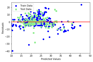
# 学習用、検証用それぞれで残差をプロット
plt.scatter(y_train_pred, y_train_pred - y_train, c = 'blue', marker = 'o', label = 'Train Data')
plt.scatter(y_test_pred, y_test_pred - y_test, c = 'lightgreen', marker = 's', label = 'Test Data')
plt.xlabel('Predicted Values')
plt.ylabel('Residuals')
# 凡例を左上に表示
plt.legend(loc = 'upper left')
# y = 0に直線を引く
plt.hlines(y = 0, xmin = -10, xmax = 50, lw = 2, color = 'red')
plt.xlim([10, 50])
plt.show()
# 平均二乗誤差を評価するためのメソッドを呼び出し
from sklearn.metrics import mean_squared_error
# 学習用、検証用データに関して平均二乗誤差を出力
print('MSE Train : %.3f, Test : %.3f' % (mean_squared_error(y_train, y_train_pred), mean_squared_error(y_test, y_test_pred)))
# 学習用、検証用データに関してR^2を出力
print('R^2 Train : %.3f, Test : %.3f' % (model.score(X_train, y_train), model.score(X_test, y_test)))
MSE Train : 44.983, Test : 40.412
R^2 Train : 0.500, Test : 0.434
考察
- 引数の型のWarningを適宜修正.
- 平均二乗誤差・R^2は学習用データ,検証用データで同等の値が得られた.
- 線形回帰は数学的に陽に解けて処理が理解しやすいが,複雑なモデルを表現できない.
