簡単に分かる正規分布

正規分布

正規分布の公式は理解するのが大変である。

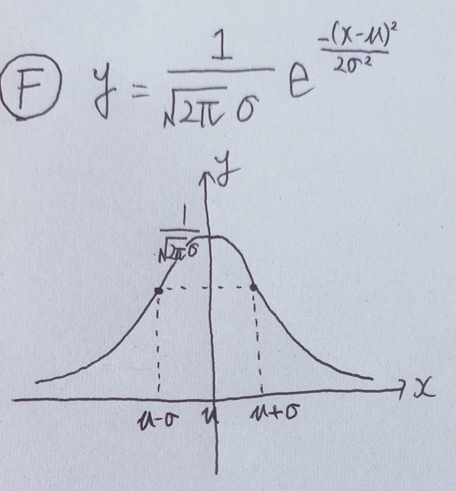
    y = \frac{1}{\sqrt{2\pi}\sigma}e^{\frac{-(x-\mu)^2}{2\sigma^2}} 

今回は、(A~F)の6つの数式を順にグラフにすることで理解しやすいです。

グラフにする数式

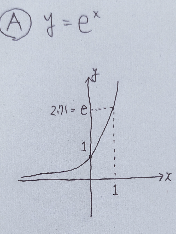
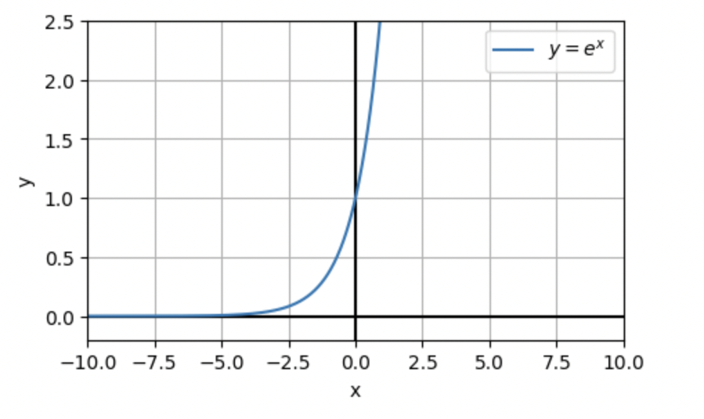
A　y = e^x 

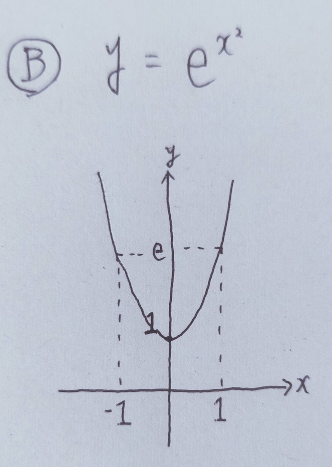
2乗で正規分布の形に近づけます。

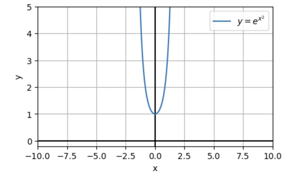
B　y = e^{x^2} 

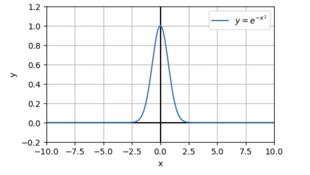
マイナスで正規分布の形に近づけます。

C　y = e^{-x^2}

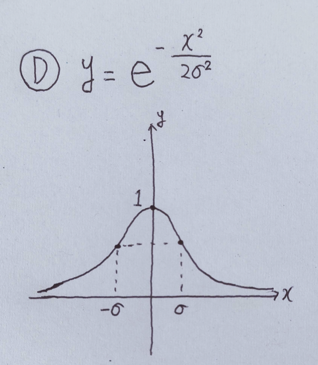
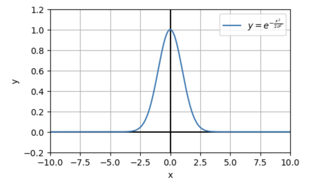
2σ^2を分母につけて正規分布の形に近づけます。

D　y = e^{\frac{-x^2}{2\sigma^2}} 

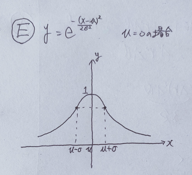
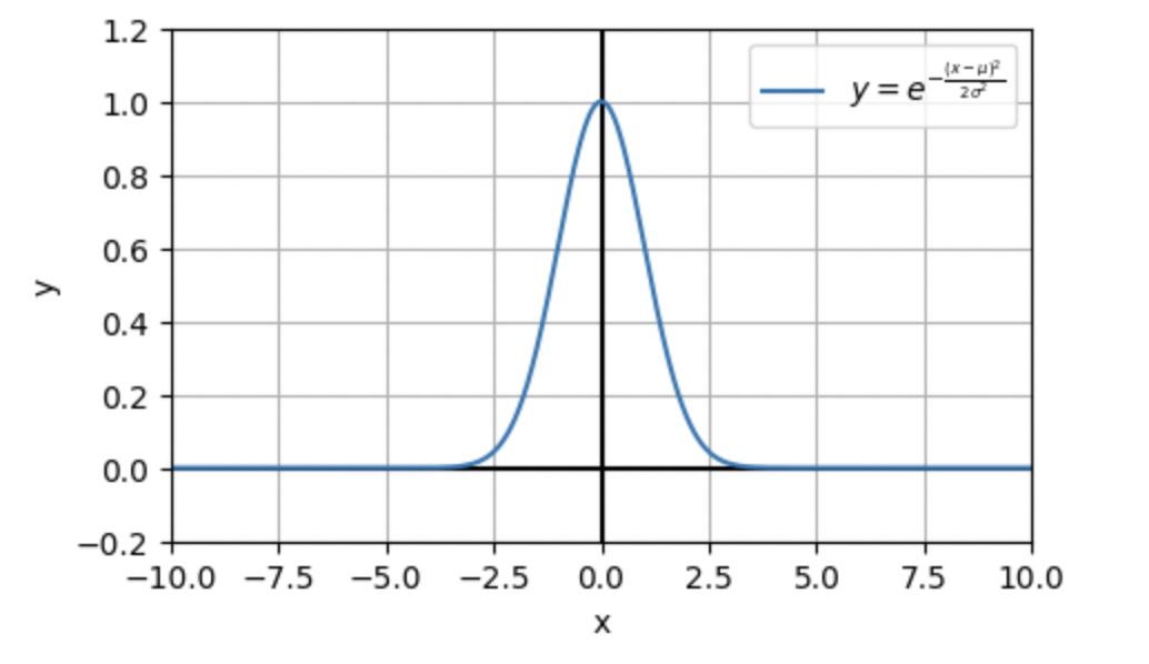
平均μをつけて正規分布の形に近づけます。

E　y = e^{\frac{-(x-\mu)^2}{2\sigma^2}} 

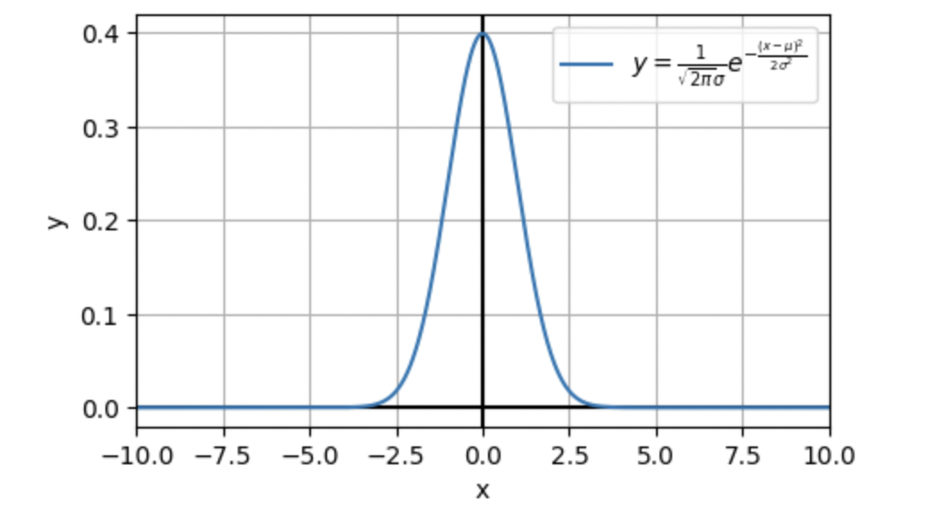
積分をして面積を1にするために係数をつけます。

F　y = \frac{1}{\sqrt{2\pi}\sigma}e^{\frac{-(x-\mu)^2}{2\sigma^2}}  

※C,Dのグラフでは変曲点を求めています。
変曲点がわからない方は下記のサイトが参考になります。

※Fでは面積が1になる証明を簡単にしています。

A

    y = e^x

B

    y = e^{x^2} 

C

    y = e^{-x^2} = \frac{1}{e^{x^2}}

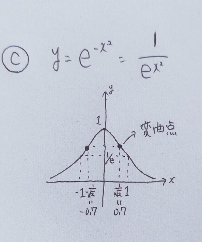
変曲点算出

\begin{align}
f(x) &= e^{-x^2}　\\
f'(x) &= -2xe^{-x^2}　\\
f''(x) &= -2e^{-x^2}・4x^2e^{-x^2}\\
&= -2e^{-x^2}(1-2x^2)\\
f''(x) &= 0より※-2e^{-x^2}は0にならないため\\
1-2x^2&=0\\
2x^2&=1\\
x^2&={\frac{1}{2}}\\
x &= \pm{\frac{1}{\sqrt2}}\\
\end{align}

※の解説
-2e^{-x^2}のxに0を代入すると
-2e^0となる。e^0=1より-2になる。

D

    y = e^{\frac{-x^2}{2\sigma^2}} 

変曲点算出

\begin{align}
f(x) &= e^{\frac{-x^2}{2\sigma^2}}\\
f'(x) &= -{\frac{2x}{2\sigma^2}} e^{\frac{-x^2}{2\sigma^2}} = -{\frac{x}{\sigma^2}} e^{\frac{-x^2}{2\sigma^2}}\\
f''(x) &= -{\frac{1}{\sigma^2}}e^{\frac{-x^2}{2\sigma^2}}-{\frac{x}{\sigma^2}}{\frac{-2x}{2\sigma^2}}e^{\frac{-x^2}{2\sigma^2}}\\
&= -{\frac{1}{\sigma^2}}e^{\frac{-x^2}{2\sigma^2}}+{\frac{x^2}{\sigma^4}}e^{\frac{-x^2}{2\sigma^2}}\\
&= -{\frac{1}{\sigma^2}}e^{\frac{-x^2}{2\sigma^2}}(1-{\frac{x^2}{\sigma^2}})\\
f''(x)&=0より\\
1-{\frac{x^2}{\sigma^2}}&=0\\
1 &= {\frac{x^2}{\sigma^2}}\\
x^2 &= \sigma^2\\
x &= \pm\sigma\\
\end{align}

E

    y = e^{\frac{-(x-\mu)^2}{2\sigma^2}} 

F

    y = \frac{1}{\sqrt{2\pi}\sigma}e^{\frac{-(x-\mu)^2}{2\sigma^2}} 

(証明)

\begin{align}
\int_{-\infty}^{\infty}f(x)dx &= 1を示す\\
\int_{-\infty}^{\infty}f(x)dx &=　\int_{-\infty}^{\infty}\frac{1}{\sqrt{2\pi}\sigma}e^{\frac{-(x-\mu)^2}{2\sigma^2}} dx　= \frac{1}{\sqrt{2\pi}\sigma}　\int_{-\infty}^{\infty}e^{\frac{-(x-\mu)^2}{2\sigma^2}}dx\\
t &= {\frac{x-\mu}{\sqrt{2}{\sigma}}}とおく。dt = {\frac{1}{\sqrt{2}{\sigma}}}dx,dx={\sqrt{2}{\sigma}}dt\\
t^2 &= {\frac{(x-\mu)}{2\sigma^2}}\\
t^2とdxを代入\\
&= \frac{1}{\sqrt{2\pi}\sigma}　\int_{-\infty}^{\infty}e^{-t^2}{\sqrt{2}{\sigma}}dt\\
&=\frac{\sqrt{2}{\sigma}}{\sqrt{2\pi}\sigma}\int_{-\infty}^{\infty}e^{-t^2}dt\\
\int_{-\infty}^{\infty}e^{-t^2}dt&=\sqrt{\pi}(ガウス積分の公式)より\\
&=\frac{\sqrt{2}{\sigma}\sqrt{\pi}}{\sqrt{2\pi}\sigma}=1\\
\end{align}

参考にした動画

Pythonでグラフを書いてみました

A　y = e^x 

import matplotlib.pyplot as plt
import numpy as np

#A
x = np.linspace(-10, 10, 1000)
y = np.exp(x)

fig, ax = plt.subplots(figsize=(5, 3), dpi=100)

plt.axhline(0, linewidth=1.5, color="black")
plt.axvline(0, linewidth=1.5, color="black")

ax.set_xlim(-10, 10)
ax.set_ylim(-0.2, 2.5)  
ax.set_xlabel("x")
ax.set_ylabel("y")

ax.plot(x, y, label=r"$y = e^x$")
ax.legend()
ax.grid()
plt.show()

B　y = e^{x^2} 

#B
x = np.linspace(-10, 10, 1000)
y = np.e ** (x ** 2)

fig, ax = plt.subplots(figsize=(5,3), dpi=100)

plt.axhline(0, linewidth=1.5, color="black")
plt.axvline(0, linewidth=1.5, color="black")

ax.set_xlim(-10, 10)
ax.set_ylim(-0.2, 5)
ax.set_xlabel("x")
ax.set_ylabel("y")

ax.plot(x, y, label=r"$y = e^{x^2}$")
ax.legend()
ax.grid()
plt.show()

C　y = e^{-x^2}

#C
x = np.linspace(-10, 10, 1000)
y = np.e ** (-1 * x ** 2)

fig, ax = plt.subplots(figsize=(5,3), dpi=100)

plt.axhline(0, linewidth=1.5, color="black")
plt.axvline(0, linewidth=1.5, color="black")

ax.set_xlim(-10, 10)
ax.set_ylim(-0.2, 1.2)
ax.set_xlabel("x")
ax.set_ylabel("y")

ax.plot(x, y, label=r"$y = e^{- x^2}$")
ax.legend()
ax.grid()
plt.show()

D　y = e^{\frac{-x^2}{2\sigma^2}} 

#D
sigma = 1  
x = np.linspace(-10, 10, 1000)
y = np.exp(-x**2 / (2 * sigma**2))

fig, ax = plt.subplots(figsize=(5, 3), dpi=100)

plt.axhline(0, linewidth=1.5, color="black")
plt.axvline(0, linewidth=1.5, color="black")

ax.set_xlim(-10, 10)
ax.set_ylim(-0.2, 1.2)
ax.set_xlabel("x")
ax.set_ylabel("y")

ax.plot(x, y, label=r"$y = e^{-\frac{x^2}{2\sigma^2}}$")
ax.legend()
ax.grid()
plt.show()

E　y = e^{\frac{-(x-\mu)^2}{2\sigma^2}} 

#E
sigma = 1
mean = 2    
x = np.linspace(-10, 10, 1000)
y = np.exp(-((x - mean)**2) / (2 * sigma**2))

fig, ax = plt.subplots(figsize=(5, 3), dpi=100)

plt.axhline(0, linewidth=1.5, color="black")
plt.axvline(0, linewidth=1.5, color="black")

ax.set_xlim(-10, 10)
ax.set_ylim(-0.2, 1.2)
ax.set_xlabel("x")
ax.set_ylabel("y")

ax.plot(x, y, label=r"$y = e^{-\frac{(x - \mu)^2}{2\sigma^2}}$")
ax.legend()
ax.grid()
plt.show()

F　y = \frac{1}{\sqrt{2\pi}\sigma}e^{\frac{-(x-\mu)^2}{2\sigma^2}}  

#F
sigma = 1
mean = 0
sigma = 1
x = np.linspace(-10, 10, 1000)
y = (1 / (np.sqrt(2 * np.pi) * sigma)) * np.exp(- (x - mean)**2 / (2 * sigma**2))

fig, ax = plt.subplots(figsize=(5, 3), dpi=100)

plt.axhline(0, linewidth=1.5, color="black")
plt.axvline(0, linewidth=1.5, color="black")

ax.set_xlim(-10, 10)
ax.set_ylim(-0.02, 0.42)
ax.set_xlabel("x")
ax.set_ylabel("y")

ax.plot(x, y, label=r"$y = \frac{1}{\sqrt{2\pi} \sigma} e^{-\frac{(x - \mu)^2}{2\sigma^2}}$")
ax.legend()
ax.grid()
plt.show()