3次元での機械学習のサンプル

この記事では、既存の機械学習を用いて3次元の空間を分類するコードを載せる。

概要

以下の2つのサイトから、引用している。

• CS231n Deep Learning for Computer Vision
  2次元の渦巻きデータから、領域分類を行う機械学習を示している。¹

• ニューラルネットのうずまきサンプル
  上記のサイトを参考にして、隠れ層を2層としている。²

今回、2つ目の記事²を参考にして、3次元のデータを学習させる。
次に、学習したニューラルネットワークが、同じ次元（3次元）の他のデータを正しく領域分類できるかを調べる。

実行環境

Ubuntu 20.04.6 LTS
python 3.8.10
git vesion 2.25.1
vscode

$ cat /etc/lsb-release 
DISTRIB_ID=Ubuntu
DISTRIB_RELEASE=20.04
DISTRIB_CODENAME=focal
DISTRIB_DESCRIPTION="Ubuntu 20.04.6 LTS"

$ python --version
Python 3.8.10

$ git --version
git version 2.25.1

$ pip list
Package                Version    
---------------------- -----------
antlr4-python3-runtime 4.9.3      
contourpy              1.1.1      
cycler                 0.12.1     
fonttools              4.56.0     
hydra-core             1.3.2      
importlib-resources    6.4.5      
kiwisolver             1.4.7      
matplotlib             3.7.5      
narwhals               1.34.0     
numpy                  1.24.4     
omegaconf              2.3.0      
packaging              24.2       
pandas                 2.0.3      
pillow                 10.4.0     
pip                    20.0.2     
pkg-resources          0.0.0      
plotly                 6.0.1      
pyparsing              3.1.4      
python-dateutil        2.9.0.post0
pytz                   2025.2     
PyYAML                 6.0.2      
setuptools             44.0.0     
six                    1.17.0     
tzdata                 2025.2     
zipp                   3.20.2     

蛇足

以下のテキストをテキストファイルに保存して、
(ファイル名なんでもいいが今回は requierments.txt)

antlr4-python3-runtime==4.9.3
contourpy==1.1.1
cycler==0.12.1
fonttools==4.56.0
hydra-core==1.3.2
importlib-resources==6.4.5
kiwisolver==1.4.7
matplotlib==3.7.5
narwhals==1.34.0
numpy==1.24.4
omegaconf==2.3.0
packaging==24.2
pandas==2.0.3
pillow==10.4.0
plotly==6.0.1
pyparsing==3.1.4
python-dateutil==2.9.0.post0
pytz==2025.2
PyYAML==6.0.2
six==1.17.0
tzdata==2025.2
zipp==3.20.2

pip install -r requirements.txt

同じライブラリを一括インストールできる。

データの作成（3次元）

　引用元の渦巻きをz方向にそのまま伸ばすとあまり拡張したことにならない。よって、3次元のデータは3重螺旋の構造をとった。

import numpy as np
import matplotlib.pyplot as plt
import plotly.express as px
import plotly.graph_objects as go
from matplotlib import cm

# Generate sample data　乱数のシード
np.random.seed(0)  # 再現性を確保するために乱数のシードを固定

# パラメータの設定
N = 30  # クラスごとのデータ点数
D = 3   # データの次元数
K = 3   # クラス数
R = 0.5 # 基本半径
R_NOISE = 0.2 # 半径に加えるノイズの強さ

# データとラベルを格納する配列を初期化
X = np.zeros((N*K, D))  # データ点の座標を格納する配列
y = np.zeros((N*K), dtype='int')  # クラスラベルを格納する配列

# 各クラスのデータを生成
for j in range(K):
    ix = range(N*j, N*(j+1))  # クラス j に対応するインデックス範囲
    r = R + np.random.randn(N) * R_NOISE  # 半径にノイズを加える
    t = np.linspace(j*2*np.pi/K, j*2*np.pi/K + 2.5*np.pi, N) + j*8*np.pi/K  # 角度（スパイラルの形状を作る）
    z = np.linspace(0.0, 2, N)  # z軸方向の値（線形に増加）

    # データ点を生成（スパイラル状に配置）
    X[ix] = np.c_[r*np.sin(t), r*np.cos(t), z]
    y[ix] = j  # クラスラベルを設定

# 3D散布図を作成
fig = px.scatter_3d(
    x = X[:, 0],  # x座標
    y = X[:, 1],  # y座標
    z = X[:, 2],  # z座標
    title = "3D Spiral Dataset",  # グラフのタイトル
    labels = {'x': 'X', 'y': 'Y', 'z': 'Z'},  # 軸ラベル
)

# グラフのレイアウトを調整
fig.update_layout(
    scene = dict(
        xaxis=dict(range = [-1.2, 1.2], nticks = 5),  # x軸の範囲と目盛り数
        yaxis=dict(range = [-1.2, 1.2], nticks = 5),  # y軸の範囲と目盛り数
        zaxis=dict(range = [-0.5, 2.5], nticks = 5),  # z軸の範囲と目盛り数
    )
)

# データ点のプロット設定
fig.update_traces(
    marker = dict(
        size = 5,  # マーカーサイズ
        color = y,  # クラスラベルに基づく色付け
        colorscale = 'jet'
    )
)

# グラフをHTMLファイルとして保存
fig.write_html('spiral_dataset_3d.html')  # 出力ファイル名

以下plotlyで出力したデータセットの図

https://ecalj.sakura.ne.jp/data/educational/spiral_dataset.html

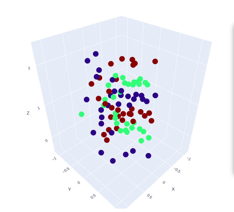
螺旋であることがわかりにくいが、螺旋になっている。
これは、螺旋構造にした後、半径方向にランダムな値を加えているためだ。

ニューラルネットワークの学習

2つ目のコードより引用した、隠れ層が2層からなるニューラルネットワークである。
この記事上では、詳しいニューラルネットワークの説明は省く。
自分が参考にした動画を以下を添付する。

https://www.youtube.com/watch?v=tc8RTtwvd5U ³
https://www.youtube.com/watch?v=0AX3KSKjyog ³
https://www.youtube.com/watch?v=SgBDx8DqBZw ³

h1 = 100 # size of hidden layer1
h2 = 50 # size of hidden layer2

#initialization
W = 0.01 * np.random.randn(D,h1)
b = np.zeros((1,h1))
W1 = 0.01 * np.random.randn(h1,h2)
b1 = np.zeros((1,h2))
W2 = 0.01 * np.random.randn(h2,K)
b2 = np.zeros((1,K))

print(' W.shape  b.shape',W.shape,b.shape)
print('W1.shape b1.shape',W1.shape,b1.shape)
print('W2.shape b2.shape',W2.shape,b2.shape)
# Set some hyperparameters
step_size = 1e-0
reg = 1e-3 # regularization strength

# Gradient descent loop
ndata = X.shape[0]
print('training data',ndata)
for i in range(1000):
  hidden_layer1 = np.maximum(0, np.dot(X, W) + b) # X ---> hidden layer1
  hidden_layer2 = np.maximum(0, np.dot(hidden_layer1, W1) + b1) # hidden layer1 ---> hidden layer2
  # evaluate class scores, [N x K]
  scores = np.dot(hidden_layer2, W2) + b2         # hidden layer2 ---> scores (logit)

  # compute the class probabilities by softmax function
  exp_scores = np.exp(scores)
  probs = exp_scores / np.sum(exp_scores, axis=1, keepdims=True) # [N x K]

  # compute the loss: average cross-entropy loss and regularization
  correct_logprobs = np.array([-np.log(probs[i,y[i]]) for i in range(ndata)]) #i番目のデータの正解確率（対数をとって−１倍する）。
  if(i==1):
    print('probs.shape=',probs.shape)
    print('corect_logprobs.shape=',correct_logprobs.shape)

  # loss function
  data_loss = np.sum(correct_logprobs)/ndata #正解確率（-logしたもの）の平均値
  reg_loss = 0.5*reg*np.sum(W*W) + 0.5*reg*np.sum(W1*W1)+ 0.5*reg*np.sum(W2*W2) #正規化関数(Wなどの値を小さくするようにする)
  loss = data_loss + reg_loss
  if i % 100 == 0:  print('iteration {}: loss {}'.format(i, loss))

  # compute the gradient on scores
  dscores = probs
  for i in range(ndata):
    dscores[i,y[i]] -= 1
  dscores /= ndata

  dW2 = np.dot(hidden_layer2.T, dscores)       # backpropate the gradient to the parameters
  db2 = np.sum(dscores, axis=0, keepdims=True) # first backprop into parameters W2 and b2

  dhidden2 = np.dot(dscores, W2.T)
  dhidden2[hidden_layer2 <= 0] = 0   # backprop the ReLU non-linearity

  dW1 = np.dot(hidden_layer1.T, dhidden2)
  db1 = np.sum(dhidden2, axis=0, keepdims=True)

  dhidden1 = np.dot(dhidden2, W1.T)
  dhidden1[hidden_layer1 <= 0] = 0

  dW = np.dot(X.T, dhidden1)
  db = np.sum(dhidden1, axis=0, keepdims=True)

  # add regularization gradient contribution
  dW2 += reg * W2
  dW1 += reg * W1
  dW += reg * W

  # perform a parameter update
  W += -step_size * dW
  b += -step_size * db
  W1 += -step_size * dW1
  b1 += -step_size * db1
  W2 += -step_size * dW2
  b2 += -step_size * db2

  # 学習済みモデルの保存
np.savez('trained_model_parameters.npz',
         W=W, b=b,
         W1=W1, b1=b1,
         W2=W2, b2=b2)

このコードで入力した3重螺旋のデータを学習させる。²

学習データの確認

領域を分類して元のデータセットに重ねて表示させる。
領域分類が正しく機能しているかを確認する。

# === 3D空間の塗り分け予測可視化（元データも重ねる） ===

# グリッド範囲と解像度
x_range = np.linspace(-1.2, 1.2, 30)
y_range = np.linspace(-1.2, 1.2, 30)
z_range = np.linspace(-0.5, 2.5, 60)
xx, yy, zz = np.meshgrid(x_range, y_range, z_range)
grid_points = np.c_[xx.ravel(), yy.ravel(), zz.ravel()]

# 各点に対して予測
h1_grid = np.maximum(0, np.dot(grid_points, W) + b)
h2_grid = np.maximum(0, np.dot(h1_grid, W1) + b1)
scores_grid = np.dot(h2_grid, W2) + b2
pred_grid = np.argmax(scores_grid, axis=1)

pred_3d = pred_grid.reshape(xx.shape)

# クラスごとの色を、matplotlibの 'jet' カラーマップで対応
unique_classes = np.unique(y)
num_classes = len(unique_classes)

# jet カラーマップから [0,1] に正規化した色を取り出す
cmap = cm.get_cmap('jet', num_classes)
class_colors = {
    cls: f'rgb({int(r*255)}, {int(g*255)}, {int(b*255)})'
    for cls, (r, g, b, _) in zip(unique_classes, cmap(np.linspace(0, 1, num_classes)))
}

# 描画用フィギュア
fig_combined = go.Figure()

# クラスごとの領域描画（Isosurface）
for cls in unique_classes:
    mask = (pred_3d == cls).astype(np.int8)
    fig_combined.add_trace(go.Isosurface(
        x = xx.ravel(), y = yy.ravel(), z = zz.ravel(),
        value = mask.ravel(),
        isomin = 0.5, isomax = 1.0,
        opacity = 0.2,
        surface_count = 1,
        colorscale = [[0, class_colors[cls]], [1, class_colors[cls]]],
        showscale = False,
        name = f"Class {cls}"
    ))

# 元の学習データ（正解ラベルに基づいて色付け）
fig_combined.add_trace(go.Scatter3d(
    x = X[:, 0], y = X[:, 1], z = X[:, 2],
    mode = 'markers',
    marker = dict(
        size = 5,
        color = y,
        colorscale = 'Jet',
        line = dict(width=0.5, color='black'),
        opacity = 1.0,
        showscale = False
    ),
    name = 'Training Data'
))

# レイアウト調整
fig_combined.update_layout(
    title = '3D Region Classification',
    scene = dict(
        xaxis = dict(range=[-1.2, 1.2]),
        yaxis = dict(range=[-1.2, 1.2]),
        zaxis = dict(range=[-0.5, 2.5])
    )
)

# 書き出し
fig_combined.write_html("spiral_net_3d_with_dataset.html")

出力したファイルが以下より

https://ecalj.sakura.ne.jp/data/educational/spiral_region_classification_with_dataset.html

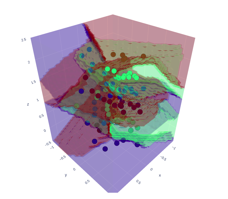
この時点での領域分類は、よくできていると言って良い。

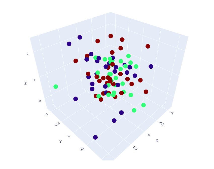
学習データを利用して他の3Dデータも試してみる。

学習したデータからパラメータを変えた他の３Dデータも試す。

import numpy as np
import plotly.graph_objects as go
import matplotlib
import plotly.express as px
from matplotlib import cm

#  ===  新しい3Dスパイラルデータを生成（あなたのコード）  === 
# Generate sample data　乱数のシード
np.random.seed(0)

N = 30 # number of points per class
D = 3 # dimensionality
K = 3 # number of classes
R = 0.5 # radius
R_NOISE = 0.4 # noise

X = np.zeros((N*K,D))
y = np.zeros((N*K),dtype = 'int')
# z = np.zeros((N*K),dtype = 'int')

for j in range(K):
  ix = range(N*j,N*(j+1))
  r = R + np.random.randn(N) * R_NOISE # radius
  t = np.linspace(j*2*np.pi/K, j*2*np.pi/K + 3*np.pi, N) + j*8*np.pi/K # theta
  z = np.linspace(0.0,2,N) 

  X[ix] = np.c_[r*np.sin(t), r*np.cos(t), z] #データ点
  y[ix] = j #正解ラベル K = 0,1,2
  # z[ix] = j #正解ラベル K = 0,1,2

fig = px.scatter_3d(
  x = X[:, 0],
  y = X[:, 1],
  z = X[:, 2],
  title = "3D Spiral Dataset",
  labels = {'x':'X','y':'Y','z':'Z'},
   )

fig.update_layout(
  scene = dict(
    xaxis = dict(range = [-1.2, 1.2], nticks = 5),
    yaxis = dict(range = [-1.2, 1.2], nticks = 5), 
    zaxis = dict(range = [-0.5, 2.5], nticks = 5), 
  )
)

fig.update_traces(
  marker = dict(
    size = 5,
    color = y,
    colorscale = 'jet'
  )
)

fig.write_html('spiral_dataset_more_ramdomly.html')


#  ===  学習済みモデルの読み込み  === 
data = np.load('trained_model_parameters.npz')
W = data['W']
b = data['b']
W1 = data['W1']
b1 = data['b1']
W2 = data['W2']
b2 = data['b2']

#  ===  新データへの順伝播による予測  === 
h1 = np.maximum(0, np.dot(X, W) + b)
h2 = np.maximum(0, np.dot(h1, W1) + b1)
scores = np.dot(h2, W2) + b2
predicted_class = np.argmax(scores, axis = 1)
accuracy = np.mean(predicted_class  ==  y)

#  ===  可視化（予測クラスによって色分け） === 
#  ===  3D空間の塗り分け予測可視化（元データも重ねる）  === 

# グリッド範囲と解像度
x_range = np.linspace(-1.2, 1.2, 30)
y_range = np.linspace(-1.2, 1.2, 30)
z_range = np.linspace(-0.5, 2.5, 60)
xx, yy, zz = np.meshgrid(x_range, y_range, z_range)
grid_points = np.c_[xx.ravel(), yy.ravel(), zz.ravel()]

# 各点に対して予測
h1_grid = np.maximum(0, np.dot(grid_points, W) + b)
h2_grid = np.maximum(0, np.dot(h1_grid, W1) + b1)
scores_grid = np.dot(h2_grid, W2) + b2
pred_grid = np.argmax(scores_grid, axis = 1)

pred_3d = pred_grid.reshape(xx.shape)
accuracy_text = f"Training Accuracy: {accuracy*100:.2f}%"

# クラスごとの色を、matplotlibの 'jet' カラーマップで対応
unique_classes = np.unique(y)
num_classes = len(unique_classes)

# jet カラーマップから [0,1] に正規化した色を取り出す
cmap = cm.get_cmap('jet', num_classes)
class_colors = {
    cls: f'rgb({int(r*255)}, {int(g*255)}, {int(b*255)})'
    for cls, (r, g, b, _) in zip(unique_classes, cmap(np.linspace(0, 1, num_classes)))
}

# 描画用フィギュア
fig_combined = go.Figure()

# クラスごとの領域描画（Isosurface）
for cls in unique_classes:
    mask = (pred_3d  ==  cls).astype(np.int8)
    fig_combined.add_trace(go.Isosurface(
        x = xx.ravel(), y = yy.ravel(), z = zz.ravel(),
        value = mask.ravel(),
        isomin = 0.5, isomax = 1.0,
        opacity = 0.2,
        surface_count = 1,
        colorscale = [[0, class_colors[cls]], [1, class_colors[cls]]],
        showscale = False,
        name = f"Class {cls}"
    ))

# 元の学習データ（正解ラベルに基づいて色付け）
fig_combined.add_trace(go.Scatter3d(
    x = X[:, 0], y = X[:, 1], z = X[:, 2],
    mode = 'markers',
    marker = dict(
        size = 5,
        color = y,
        colorscale = 'Jet',
        line = dict(width = 0.5, color = 'black'),
        opacity = 1.0,
        showscale = False
    ),
    name = 'Training Data'
))

# レイアウト調整
fig_combined.update_layout(
    title = '3D Region Coloring with Class-Matched Colors',
    scene = dict(
        xaxis = dict(range = [-1.2, 1.2]),
        yaxis = dict(range = [-1.2, 1.2]),
        zaxis = dict(range = [-0.5, 2.5])
    )
)

# 書き出し
fig_combined.write_html("spiral_region_classification_more_ramdomly.html")

作成したデータセット及び領域分類も重ねて表示した結果が以下

https://ecalj.sakura.ne.jp/data/educational/spiral_dataset_more_ramdomly.html

https://ecalj.sakura.ne.jp/data/educational/spiral_region_classification_more_ramdomly.html

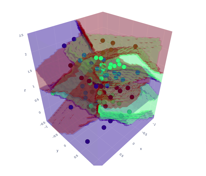
これも分類がうまくできている。

まとめ

本記事では、ニューラルネットワークを用いた3次元空間の分類問題について、以下のステップを通して紹介した。

• 2次元の渦巻きデータ（spiral）の生成と分類（引用）

• その拡張として3次元スパイラルデータの生成

• ニューラルネットワークによる分類と学習の実装

• Plotlyを用いた3D空間上での可視化（分類結果の重ね描き）

2025/04/24以降にすること

• スパイラルにこだわらず、3次元の他のデータで領域分類が可能化を調べる。
• どの程度分類できているかの指標が明確ではない。したがって、指標を作成し掲載する。
• コードの見直しと、githubに追加する。
  • クラス、関数を実装して、拡張しやすいように
  • パラメータファイルを用意して、学習効率を良くする
  • 学習部分をpytorchに書き換えて、実装する

vscode関連

仮想環境を作成（vscodeで対象ディレクトリを開いておく）

python3 -m venv your_env_name

仮想環境を有効化

source your_env_name/bin/activate

使用中ライブラリとバージョンを記録

pip freeze > requirements.txt

記録されたライブラリを一括インストール

pip install -r requirements.txt

仮想環境ディレクトリはリモートにpushしないよう記述

.gitignore

仮想環境を終了

deactivate

ライブラリのインストール方法（明示的にPython3を指定）

python3 -m pip install package_name

全体コード

import numpy as np
import matplotlib.pyplot as plt
import plotly.express as px
import plotly.graph_objects as go
from matplotlib import cm

# Generate sample data　乱数のシード
np.random.seed(0)  # 再現性を確保するために乱数のシードを固定

# パラメータの設定
N = 30  # クラスごとのデータ点数
D = 3   # データの次元数
K = 3   # クラス数
R = 0.5 # 基本半径
R_NOISE = 0.2 # 半径に加えるノイズの強さ

# データとラベルを格納する配列を初期化
X = np.zeros((N*K, D))  # データ点の座標を格納する配列
y = np.zeros((N*K), dtype='int')  # クラスラベルを格納する配列

# 各クラスのデータを生成
for j in range(K):
    ix = range(N*j, N*(j+1))  # クラス j に対応するインデックス範囲
    r = R + np.random.randn(N) * R_NOISE  # 半径にノイズを加える
    t = np.linspace(j*2*np.pi/K, j*2*np.pi/K + 2.5*np.pi, N) + j*8*np.pi/K  # 角度（スパイラルの形状を作る）
    z = np.linspace(0.0, 2, N)  # z軸方向の値（線形に増加）

    # データ点を生成（スパイラル状に配置）
    X[ix] = np.c_[r*np.sin(t), r*np.cos(t), z]
    y[ix] = j  # クラスラベルを設定

# 3D散布図を作成
fig = px.scatter_3d(
    x=X[:, 0],  # x座標
    y=X[:, 1],  # y座標
    z=X[:, 2],  # z座標
    title="3D Spiral Dataset",  # グラフのタイトル
    labels={'x': 'X', 'y': 'Y', 'z': 'Z'},  # 軸ラベル
)

# グラフのレイアウトを調整
fig.update_layout(
    scene=dict(
        xaxis=dict(range=[-1.2, 1.2], nticks=5),  # x軸の範囲と目盛り数
        yaxis=dict(range=[-1.2, 1.2], nticks=5),  # y軸の範囲と目盛り数
        zaxis=dict(range=[-0.5, 2.5], nticks=5),  # z軸の範囲と目盛り数
    )
)

# データ点のプロット設定
fig.update_traces(
    marker=dict(
        size=5,  # マーカーサイズ
        color=y,  # クラスラベルに基づく色付け
        colorscale='jet'
    )
)

# グラフをHTMLファイルとして保存
fig.write_html('spiral_dataset_3d.html')  # 出力ファイル名

# NN Architecture input, hidden1, hidden2
#  input X -->W,b-->ReLU--> hidden layer1 -->W1,b1-->ReLU=> hidden layer2 -->W2,b2---> scores
# initialize parameters randomly
h1 = 100 # size of hidden layer1
h2 = 50 # size of hidden layer2

#initialization
W = 0.01 * np.random.randn(D,h1)
b = np.zeros((1,h1))
W1 = 0.01 * np.random.randn(h1,h2)
b1 = np.zeros((1,h2))
W2 = 0.01 * np.random.randn(h2,K)
b2 = np.zeros((1,K))

print(' W.shape  b.shape',W.shape,b.shape)
print('W1.shape b1.shape',W1.shape,b1.shape)
print('W2.shape b2.shape',W2.shape,b2.shape)
# Set some hyperparameters
step_size = 1e-0
reg = 1e-3 # regularization strength

# Gradient descent loop
ndata = X.shape[0]
print('training data',ndata)
for i in range(1000):
  hidden_layer1 = np.maximum(0, np.dot(X, W) + b) # X ---> hidden layer1
  hidden_layer2 = np.maximum(0, np.dot(hidden_layer1, W1) + b1) # hidden layer1 ---> hidden layer2
  # evaluate class scores, [N x K]
  scores = np.dot(hidden_layer2, W2) + b2         # hidden layer2 ---> scores (logit)

  # compute the class probabilities by softmax function
  exp_scores = np.exp(scores)
  probs = exp_scores / np.sum(exp_scores, axis=1, keepdims=True) # [N x K]

  # compute the loss: average cross-entropy loss and regularization
  correct_logprobs = np.array([-np.log(probs[i,y[i]]) for i in range(ndata)]) #i番目のデータの正解確率（対数をとって−１倍する）。
  if(i==1):
    print('probs.shape=',probs.shape)
    print('corect_logprobs.shape=',correct_logprobs.shape)

  # loss function
  data_loss = np.sum(correct_logprobs)/ndata #正解確率（-logしたもの）の平均値
  reg_loss = 0.5*reg*np.sum(W*W) + 0.5*reg*np.sum(W1*W1)+ 0.5*reg*np.sum(W2*W2) #正規化関数(Wなどの値を小さくするようにする)
  loss = data_loss + reg_loss
  if i % 100 == 0:  print('iteration {}: loss {}'.format(i, loss))

  # compute the gradient on scores
  dscores = probs
  for i in range(ndata):
    dscores[i,y[i]] -= 1
  dscores /= ndata

  dW2 = np.dot(hidden_layer2.T, dscores)       # backpropate the gradient to the parameters
  db2 = np.sum(dscores, axis=0, keepdims=True) # first backprop into parameters W2 and b2

  dhidden2 = np.dot(dscores, W2.T)
  dhidden2[hidden_layer2 <= 0] = 0   # backprop the ReLU non-linearity

  dW1 = np.dot(hidden_layer1.T, dhidden2)
  db1 = np.sum(dhidden2, axis=0, keepdims=True)

  dhidden1 = np.dot(dhidden2, W1.T)
  dhidden1[hidden_layer1 <= 0] = 0

  dW = np.dot(X.T, dhidden1)
  db = np.sum(dhidden1, axis=0, keepdims=True)

  # add regularization gradient contribution
  dW2 += reg * W2
  dW1 += reg * W1
  dW += reg * W

  # perform a parameter update
  W += -step_size * dW
  b += -step_size * db
  W1 += -step_size * dW1
  b1 += -step_size * db1
  W2 += -step_size * dW2
  b2 += -step_size * db2

"""学習終了。以下で学習したNNによりすべての点での値を予想する（塗り分けることになる）"""


"""平面上でのすべての点での予想をおこなった。なるほど、うまく予想している。"""

# === 3D空間の塗り分け予測可視化（元データも重ねる） ===

# グリッド範囲と解像度
x_range = np.linspace(-1.2, 1.2, 30)
y_range = np.linspace(-1.2, 1.2, 30)
z_range = np.linspace(-0.5, 2.5, 60)
xx, yy, zz = np.meshgrid(x_range, y_range, z_range)
grid_points = np.c_[xx.ravel(), yy.ravel(), zz.ravel()]

# 各点に対して予測
h1_grid = np.maximum(0, np.dot(grid_points, W) + b)
h2_grid = np.maximum(0, np.dot(h1_grid, W1) + b1)
scores_grid = np.dot(h2_grid, W2) + b2
pred_grid = np.argmax(scores_grid, axis=1)

pred_3d = pred_grid.reshape(xx.shape)

# クラスごとの色を、matplotlibの 'jet' カラーマップで対応
unique_classes = np.unique(y)
num_classes = len(unique_classes)

# jet カラーマップから [0,1] に正規化した色を取り出す
cmap = cm.get_cmap('jet', num_classes)
class_colors = {
    cls: f'rgb({int(r*255)}, {int(g*255)}, {int(b*255)})'
    for cls, (r, g, b, _) in zip(unique_classes, cmap(np.linspace(0, 1, num_classes)))
}

# 描画用フィギュア
fig_combined = go.Figure()

# クラスごとの領域描画（Isosurface）
for cls in unique_classes:
    mask = (pred_3d == cls).astype(np.int8)
    fig_combined.add_trace(go.Isosurface(
        x=xx.ravel(), y=yy.ravel(), z=zz.ravel(),
        value=mask.ravel(),
        isomin=0.5, isomax=1.0,
        opacity=0.2,
        surface_count=1,
        colorscale=[[0, class_colors[cls]], [1, class_colors[cls]]],
        showscale=False,
        name=f"Class {cls}"
    ))

# 元の学習データ（正解ラベルに基づいて色付け）
fig_combined.add_trace(go.Scatter3d(
    x=X[:, 0], y=X[:, 1], z=X[:, 2],
    mode='markers',
    marker=dict(
        size=5,
        color=y,
        colorscale='Jet',
        line=dict(width=0.5, color='black'),
        opacity=1.0,
        showscale=False
    ),
    name='Training Data'
))

# レイアウト調整
fig_combined.update_layout(
    title='3D Region Coloring with Class-Matched Colors',
    scene=dict(
        xaxis=dict(range=[-1.2, 1.2]),
        yaxis=dict(range=[-1.2, 1.2]),
        zaxis=dict(range=[-0.5, 2.5])
    )
)

# 書き出し
fig_combined.write_html("spiral_net_3d_with_matched_colors.html")

1. Stanford CS231n: https://cs231n.github.io/neural-networks-case-study/ ↩

2. Qiita記事「ニューラルネットのうずまきサンプル」: https://qiita.com/takaokotani/items/ed5b02dc3e7ae75e6002 ↩ ↩² ↩³

3. https://www.youtube.com/@3Blue1BrownJapan ↩ ↩² ↩³