1. はじめに
Python機械学習プログラミング[第2版] という本を買って勉強を始めました。効果的な学習を進める為には、勉強した内容をアウトプットするのが効果的ということで、勉強した内容を備忘録の形でここに残すことを進めています。
なお、本ではコードを一部 jupyter notebook形式で記載しているようですが、ここでは.py形式でも実行できるような形式で記載したいと思います。
今回は、第2章のADALINEについて、
2. ADALINE
ADALINEとは、二乗誤差(目標値と予測値の差の二乗)をコスト関数として、勾配降下法を使ってコスト関数を最小化する重みを見つける手法です。
早速、コードを動かしてみると、
import numpy as np
import pandas as pd
import matplotlib.pyplot as plt

class AdalineGD(object):

    def __init__(self, eta=0.01, n_iter=50, random_state=1):
        self.eta = eta
        self.n_iter = n_iter
        self.random_state = random_state

    def fit(self, X, y):

        rgen = np.random.RandomState(self.random_state)
        self.w_ = rgen.normal(loc=0.0, scale=0.01, size=1 + X.shape[1])
        self.cost_ = []

        for i in range(self.n_iter):
            net_input = self.net_input(X)
            output = self.activation(net_input)
            errors = (y - output)
            self.w_[1:] += self.eta * X.T.dot(errors)
            self.w_[0] += self.eta * errors.sum()
            cost = (errors**2).sum() / 2.0
            self.cost_.append(cost)
        return self

    def net_input(self, X):
        return np.dot(X, self.w_[1:]) + self.w_[0]

    def activation(self, X):
        return X

    def predict(self, X):
        return np.where(self.activation(self.net_input(X)) >= 0.0, 1, -1)

# Iris データセットの読み込みと加工
df = pd.read_csv('https://archive.ics.uci.edu/ml/'
        'machine-learning-databases/iris/iris.data', header=None)
y = df.iloc[0:100, 4].values
y = np.where(y == 'Iris-setosa', -1, 1)
X = df.iloc[0:100, [0, 2]].values


# 学習率を変化させた場合のコストグラフ比較
fig, ax = plt.subplots(nrows=1, ncols=2, figsize=(10, 4))

ada1 = AdalineGD(n_iter=10, eta=0.01).fit(X, y)
ax[0].plot(range(1, len(ada1.cost_) + 1), np.log10(ada1.cost_), marker='o')
ax[0].set_xlabel('Epochs')
ax[0].set_ylabel('log(Sum-squared-error)')
ax[0].set_title('Adaline - Learning rate 0.01')

ada2 = AdalineGD(n_iter=10, eta=0.0001).fit(X, y)
ax[1].plot(range(1, len(ada2.cost_) + 1), ada2.cost_, marker='o')
ax[1].set_xlabel('Epochs')
ax[1].set_ylabel('Sum-squared-error')
ax[1].set_title('Adaline - Learning rate 0.0001')

plt.show()
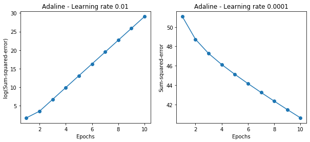
1Epochs毎に、データセット全体の二乗誤差を計算し、重みを更新しています。
ここで本が言いたいのは、学習率が大きい(Learinig rate 0.01)とロス関数は逆に大きくなってしまい、学習率が小さい(Learning rate 0.0001)とロス関数はゆっくりとしか下がらないということで、それは良く分かります。
ただ、コードの中身がピンと来ない。特に、self.w_[1:] += self.eta * X.T.dot(errors)とか、何をやっているのか良く分からない。
ということで、今回はデータセットや重みの初期値を単純化して、コードの内容を良く理解してみます。
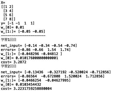
(データセットと重みの初期値)
X = np.array([[1, 2],[3, 4], [5, 6], [7, 8]])
y = np.array([-1, -1, 1, 1])
w = [0.01, -0.05, -0.05]
*X, yのデータはたった4個、wの初期値も見える化しました
では、この設定で変数がどう変化しているのかモニターする為に、先ほどのコードを改造して動かしてみます。なお、グラフ表示は Learning rate 0.0001のみとします。
import numpy as np
import matplotlib.pyplot as plt

class AdalineGD(object):

    def __init__(self, eta=0.01, n_iter=50, random_state=1):
        self.eta = eta
        self.n_iter = n_iter
        self.random_state = random_state

    def fit(self, X, y):
        self.w_ = np.array([0.01, -0.05, -0.05]) # 重みの設定
        print('w_[0]=',self.w_[0])
        print('w_[1:]=', self.w_[1:])
        print('---------------------')

        self.cost_ = []

        for i in range(self.n_iter):
            net_input = self.net_input(X)
            output = self.activation(net_input)
            errors = (y - output)
            self.w_[1:] += self.eta * X.T.dot(errors)
            self.w_[0] += self.eta * errors.sum()
            cost = (errors**2).sum() / 2.0
            self.cost_.append(cost)
            # ---------------------------------- モニター ↓
            print('学習'+str(i+1)+'回目')
            print('net_input=', net_input)
            print('errors=', errors)
            print('w_[1:]=', self.w_[1:])
            print('w_[0]=', self.w_[0])
            print('cost=', cost)
            # ---------------------------------  モニター ↑
        return self

    def net_input(self, X):
        return np.dot(X, self.w_[1:]) + self.w_[0]

    def activation(self, X):
        return X

    def predict(self, X):
        return np.where(self.activation(self.net_input(X)) >= 0.0, 1, -1)

# データセット
X = np.array([[1, 2],[3, 4],[5, 6],[7, 8]])
y = np.array([-1, -1, 1, 1])
print('X=')
print(X)
print('y=', y)

# コストグラフ
ada = AdalineGD(n_iter=10, eta=0.0001).fit(X, y)
plt.plot(range(1, len(ada.cost_)+1), ada.cost_, marker='o')
plt.xlabel('Epochs')
plt.ylabel('Sum-squared-error')
plt.title('Adaline - Learning rate 0.0001')
plt.show()
・・・・・・・・・・ 中略 ・・・・・・・・・・
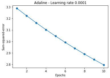
とりあえず、たった4個のデータでも、ちゃんと動くようです。それでは、学習1回目だけの結果を元に、何をやっているのか、具体的に確認してみましょう。
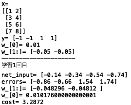
net_input = np.dot(X, w_[1:]) + w_[0]
= [1*-0.05+2*-0.05、 3*-0.05+4*-0.05、 5*-0.05+6*-0.05、 7*-0.05+8*-0.05] + 0.01
= [-0.15 -0.35 -0.55 -0.75] + 0.01 = [-0.14 -0.34 -0.54 -0.74]
*Xが1行2列が4個、w_[1:]が1行2列なので、np.dotの内積計算を使っています。
errors = y - output = y - net_input
= [ -1-(-0.14)、-1-(-0.34)、1-(-0.54)、1-(-0.74)] = [-0.86 -0.66 1.54 1.74]
*activationがダミーなので、output = net_input
w_[1:] = w_[1:] + ( eta * X.T.dot(errors))
= [-0.05 -0.05] + (0.0001 * [1*-0.86+3*-0.66+51.54+71.74、 2*-0.86+4*-0.66+61.54+81.74])
= [-0.05 -0.05] + (0.0001 * [17.04 18.8])
= [-0.05 -0.05] + [0.001704 0.00188]
= [-0.048296 -0.04812]
*Xが1行2列が4個、errorsが1行4列なので、Xを2行4列に転置して、np.dotの内積計算を行っているようです。
w_[0] = w_[0] + eta * errors.sum()
= 0.01 + (0.0001*-0.86+ 0.0001*-0.66+ 0.00011.54+ 0.0001 1.74)
= 0.010176
チェック完了!
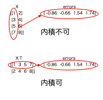
つまり、Xの転置を行っているのは、numpyの内積を使う為なのです。もう1つ、np.dotでないのに内積が出来るかですが、実際にコードを書いて確認してみましょう。
import numpy as np
X = np.array([[1, 2], [3, 4], [5, 6], [7, 8]])
errors = np.array([-0.86,-0.66,1.54,1.74])
print('X.T.dot(errors)=', X.T.dot(errors))
print('np.dot(X.T, errors)=', np.dot(X.T, errors))

# 出力
X.T.dot(errors)= [17.04 18.8 ]
np.dot(X.T, errors)= [17.04 18.8 ]
そうすると、確かに X.T.dot(errors)は、np.dot(X.T, errors)と同じ結果になります。Webで色々調べてみると、npと書かなくてもnp.dotであることが明らかな場合は、npは省略しても良いらしいです。
えー何それ。ちょっとコードの書き方に文句があります。Webで色々調べましたが、ほとんどの場合は、np.dot(X.T, errors)の方で表記がされていました。初学者がつまらない所で迷わない様に、第3版では、ぜひnp.dot(X.T, errors)に直して欲しいです(笑)。冗談ですが。
さて、今度はデータの標準化です。これは、データを平均0、標準偏差1に変換することで、学習コストの収束を早めようということです。早速、テキストに載っているコードを動かすと、
import numpy as np
import pandas as pd
import matplotlib.pyplot as plt
from matplotlib.colors import ListedColormap

def plot_decision_regions(X, y, classifier, resolution=0.02):

    # setup marker generator and color map
    markers = ('s', 'x', 'o', '^', 'v')
    colors = ('red', 'blue', 'lightgreen', 'gray', 'cyan')
    cmap = ListedColormap(colors[:len(np.unique(y))])

    # plot the decision surface
    x1_min, x1_max = X[:, 0].min() - 1, X[:, 0].max() + 1
    x2_min, x2_max = X[:, 1].min() - 1, X[:, 1].max() + 1
    xx1, xx2 = np.meshgrid(np.arange(x1_min, x1_max, resolution),
                           np.arange(x2_min, x2_max, resolution))
    Z = classifier.predict(np.array([xx1.ravel(), xx2.ravel()]).T)
    Z = Z.reshape(xx1.shape)
    plt.contourf(xx1, xx2, Z, alpha=0.3, cmap=cmap)
    plt.xlim(xx1.min(), xx1.max())
    plt.ylim(xx2.min(), xx2.max())

    # plot class samples
    for idx, cl in enumerate(np.unique(y)):
        plt.scatter(x=X[y == cl, 0],
                    y=X[y == cl, 1],
                    alpha=0.8,
                    c=colors[idx],
                    marker=markers[idx],
                    label=cl,
                    edgecolor='black')


class AdalineGD(object):

    def __init__(self, eta=0.01, n_iter=50, random_state=1):
        self.eta = eta
        self.n_iter = n_iter
        self.random_state = random_state

    def fit(self, X, y):
        rgen = np.random.RandomState(self.random_state)
        self.w_ = rgen.normal(loc=0.0, scale=0.01, size=1 + X.shape[1])
        self.cost_ = []

        for i in range(self.n_iter):
            net_input = self.net_input(X)
            output = self.activation(net_input)
            errors = (y - output)
            self.w_[1:] += self.eta * X.T.dot(errors)
            self.w_[0] += self.eta * errors.sum()
            cost = (errors**2).sum() / 2.0
            self.cost_.append(cost)
        return self

    def net_input(self, X):
        return np.dot(X, self.w_[1:]) + self.w_[0]

    def activation(self, X):
        return X

    def predict(self, X):
        return np.where(self.activation(self.net_input(X)) >= 0.0, 1, -1)


# データセット読み込み
df = pd.read_csv('https://archive.ics.uci.edu/ml/'
        'machine-learning-databases/iris/iris.data', header=None)
y = df.iloc[0:100, 4].values
y = np.where(y == 'Iris-setosa', -1, 1)
X = df.iloc[0:100, [0, 2]].values

# ---------- データの標準化 ------------
X_std = np.copy(X)  # Xをコピー
X_std[:, 0] = (X[:, 0] - X[:, 0].mean()) / X[:, 0].std()  # x[0]の標準化
X_std[:, 1] = (X[:, 1] - X[:, 1].mean()) / X[:, 1].std()  # x[1]の標準化
# -----------------------------------

# 学習
ada = AdalineGD(n_iter=15, eta=0.01)
ada.fit(X_std, y)

# 学習コストグラフ表示
plot_decision_regions(X_std, y, classifier=ada)
plt.title('Adaline - Gradient Descent')
plt.xlabel('sepal length [standardized]')
plt.ylabel('petal length [standardized]')
plt.legend(loc='upper left')
plt.tight_layout()
plt.show()

# 決定領域グラフ表示
plt.plot(range(1, len(ada.cost_) + 1), ada.cost_, marker='o')
plt.xlabel('Epochs')
plt.ylabel('Sum-squared-error')
plt.tight_layout()
plt.show()
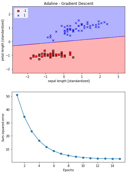
凄い! 学習率(eta)が0.01の時、Xデータがそのままの場合は学習コストグラフが増えてしまいましたが、Xデータを標準化すると素早く学習コストが0に向かって低減しています。そして、決定領域グラフもちゃんと描けています。
何が変わったのかと言えば、Xデータを標準化しただけです。データの標準化による効果は絶大ですね。
さて、Irisの様な極めて小さなデータセットならいざ知らず、機械学習に使われるデータセットは非常に大きなものなので、毎回データセット単位で重みを更新していては、莫大な計算が必要となり現実的ではありません。
そこで、データをシャッフルして、データ1つ毎にコストを計算し重みを更新しようという手法があり、これを確率的勾配法と言います。
テキストのコードを動かしてみましょう。
import numpy as np
import pandas as pd
import matplotlib.pyplot as plt
from matplotlib.colors import ListedColormap

def plot_decision_regions(X, y, classifier, resolution=0.02):

    # setup marker generator and color map
    markers = ('s', 'x', 'o', '^', 'v')
    colors = ('red', 'blue', 'lightgreen', 'gray', 'cyan')
    cmap = ListedColormap(colors[:len(np.unique(y))])

    # plot the decision surface
    x1_min, x1_max = X[:, 0].min() - 1, X[:, 0].max() + 1
    x2_min, x2_max = X[:, 1].min() - 1, X[:, 1].max() + 1
    xx1, xx2 = np.meshgrid(np.arange(x1_min, x1_max, resolution),
                           np.arange(x2_min, x2_max, resolution))
    Z = classifier.predict(np.array([xx1.ravel(), xx2.ravel()]).T)
    Z = Z.reshape(xx1.shape)
    plt.contourf(xx1, xx2, Z, alpha=0.3, cmap=cmap)
    plt.xlim(xx1.min(), xx1.max())
    plt.ylim(xx2.min(), xx2.max())

    # plot class samples
    for idx, cl in enumerate(np.unique(y)):
        plt.scatter(x=X[y == cl, 0],
                    y=X[y == cl, 1],
                    alpha=0.8,
                    c=colors[idx],
                    marker=markers[idx],
                    label=cl,
                    edgecolor='black')

# ## Large scale machine learning and stochastic gradient descent
class AdalineSGD(object):

    def __init__(self, eta=0.01, n_iter=10, shuffle=True, random_state=None):
        self.eta = eta
        self.n_iter = n_iter
        self.w_initialized = False
        self.shuffle = shuffle
        self.random_state = random_state

    def fit(self, X, y):
        self._initialize_weights(X.shape[1])
        self.cost_ = []
        for i in range(self.n_iter):
            if self.shuffle:
                X, y = self._shuffle(X, y)
            cost = []
            for xi, target in zip(X, y):
                cost.append(self._update_weights(xi, target))
            avg_cost = sum(cost) / len(y)
            self.cost_.append(avg_cost)
        return self

    def partial_fit(self, X, y):
        if not self.w_initialized:
            self._initialize_weights(X.shape[1])
        if y.ravel().shape[0] > 1:
            for xi, target in zip(X, y):
                self._update_weights(xi, target)
        else:
            self._update_weights(X, y)
        return self

    def _shuffle(self, X, y):
        r = self.rgen.permutation(len(y))
        return X[r], y[r]

    def _initialize_weights(self, m):
        self.rgen = np.random.RandomState(self.random_state)
        self.w_ = self.rgen.normal(loc=0.0, scale=0.01, size=1 + m)
        self.w_initialized = True

    def _update_weights(self, xi, target):
        output = self.activation(self.net_input(xi))
        error = (target - output)
        self.w_[1:] += self.eta * xi.dot(error)
        self.w_[0] += self.eta * error
        cost = 0.5 * error**2
        return cost

    def net_input(self, X):
        return np.dot(X, self.w_[1:]) + self.w_[0]

    def activation(self, X):
        return X

    def predict(self, X):
        return np.where(self.activation(self.net_input(X)) >= 0.0, 1, -1)


df = pd.read_csv('https://archive.ics.uci.edu/ml/'
        'machine-learning-databases/iris/iris.data', header=None)
y = df.iloc[0:100, 4].values
y = np.where(y == 'Iris-setosa', -1, 1)
X = df.iloc[0:100, [0, 2]].values


# ## Improving gradient descent through feature scaling
# standardize features
X_std = np.copy(X)
X_std[:, 0] = (X[:, 0] - X[:, 0].mean()) / X[:, 0].std()
X_std[:, 1] = (X[:, 1] - X[:, 1].mean()) / X[:, 1].std()


ada = AdalineSGD(n_iter=15, eta=0.01, random_state=1)
ada.fit(X_std, y)

plot_decision_regions(X_std, y, classifier=ada)
plt.title('Adaline - Stochastic Gradient Descent')
plt.xlabel('sepal length [standardized]')
plt.ylabel('petal length [standardized]')
plt.legend(loc='upper left')
plt.tight_layout()
plt.show()

plt.plot(range(1, len(ada.cost_) + 1), ada.cost_, marker='o')
plt.xlabel('Epochs')
plt.ylabel('Average Cost')
plt.tight_layout()
plt.show()
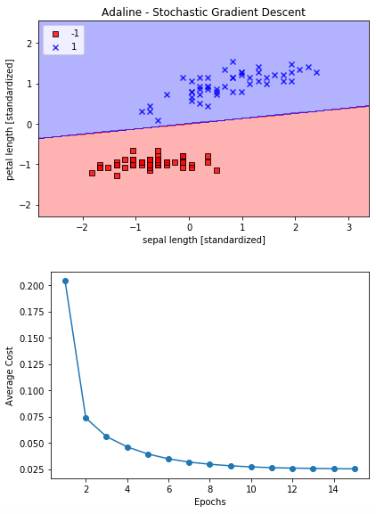
素晴らしい! コストグラフの低減効果が桁違いに早い(1Epochsの時点で、前回50、今回0.2)、爆速です。
ただ、余計な機能が入っているので、コードが少し分かり難いです。それは、オンライン機能(def pertial_fit(self, X, y):)です。
オンラインで新たなデータが追加される度に学習することを考えると、ご破算にして最初から学習するより、重みの初期化を行わず今までの重みを生かして、新たなデータのみで学習させるからです。これに伴い、重みの初期化機能(def _shuffle(self, X, y):)も独立させています。
このオンライン機能は、この章では実際に使っていないので、コードでは省いておいた方が分かり易い様な気がします。
コードのポイントは、データセットの順番を並び替えるところ、
    def _shuffle(self, X, y):
        r = self.rgen.permutation(len(y))
        print(len(y))
        return X[r], y[r]
データをシャッフルするには、np.random.shuffle() と np.random.permutation()があるのですが、shuffle()は元データを並び替え、permutation() は並び替えたデータのコピーを生成します。Epochs毎にデータセットをシャッフルするのには、permutation()の方が都合が良いので、こちらを使っている様です。
後、self.rgen = np.random.RandomState(self.random_state)なので、シードを使って再現性のあるシャッフルを実現しています。
サンプルでも確認してみましょう。
X = np.array([[1, 2], [3, 4], [5, 6], [7, 8]])
y = np.array([-1, -1, 1, 1])
print(X)
print(y)

def shuffle(X, y):
    r = np.random.RandomState(3).permutation(len(y))
    return X[r], y[r]

X_s, y_s = shuffle(X, y)
print(X_s)
print(y_s)

# 出力
[[1 2]
 [3 4]
 [5 6]
 [7 8]]
[-1 -1  1  1]
[[7 8]
 [3 4]
 [1 2]
 [5 6]]
[ 1 -1 -1  1]
サンプル(シード4)で試してみると、こんな感じ。データのシャッフルには便利そうです。
もう1つのポイントは、def fit(self, X, y):のところ
    def fit(self, X, y):
        self._initialize_weights(X.shape[1])
        self.cost_ = []
        for i in range(self.n_iter):
            if self.shuffle:  # シャッフル指定があればシャッフル
                X, y = self._shuffle(X, y)  # データセットのシャッフル
            cost = []
            for xi, target in zip(X, y):
                cost.append(self._update_weights(xi, target))  # 重みの更新
            avg_cost = sum(cost) / len(y)  # Epochs毎に平均コストを算出
            self.cost_.append(avg_cost)  # 平均コストを保存
        return self
今回は、1つのデータ毎にコストを計算し重みを更新して、1Epochs分終わったら平均コストを算出しています。後は、書き方は違いますが、内容は一緒です。
さて、せっかくですので、シャッフルの効果を見て見ましょうか。シャッフルした場合とシャッフルしない場合の学習コストを同じグラフに描かせるコードにして、結果を見てみましょう。きっと、歴然とした差があるはずですので、
シャッフルするかどうかは、ada = AdalineSGD(n_iter=15, eta=0.01, shuffle=False, random_state=1) でインスタンス化する時に、shuffle= で記載することで指定出来ます。
import numpy as np
import pandas as pd
import matplotlib.pyplot as plt

# ## Large scale machine learning and stochastic gradient descent
class AdalineSGD(object):

    def __init__(self, eta=0.01, n_iter=10, shuffle=True, random_state=None):
        self.eta = eta
        self.n_iter = n_iter
        self.w_initialized = False
        self.shuffle = shuffle
        self.random_state = random_state

    def fit(self, X, y):
        self._initialize_weights(X.shape[1])
        self.cost_ = []
        self.cost_d = []  ###
        for i in range(self.n_iter):
            if self.shuffle:
                X, y = self._shuffle(X, y)
            cost = []
            for xi, target in zip(X, y):
                cost.append(self._update_weights(xi, target))
                self.cost_d.append(self._update_weights(xi, target))
            avg_cost = sum(cost) / len(y)
            self.cost_.append(avg_cost)
        return self

    def partial_fit(self, X, y):
        if not self.w_initialized:
            self._initialize_weights(X.shape[1])
        if y.ravel().shape[0] > 1:
            for xi, target in zip(X, y):
                self._update_weights(xi, target)
        else:
            self._update_weights(X, y)
        return self

    def _shuffle(self, X, y):
        r = self.rgen.permutation(len(y))
        return X[r], y[r]

    def _initialize_weights(self, m):
        self.rgen = np.random.RandomState(self.random_state)
        self.w_ = self.rgen.normal(loc=0.0, scale=0.01, size=1 + m)
        self.w_initialized = True

    def _update_weights(self, xi, target):
        output = self.activation(self.net_input(xi))
        error = (target - output)
        self.w_[1:] += self.eta * xi.dot(error)
        self.w_[0] += self.eta * error
        cost = 0.5 * error**2
        return cost

    def net_input(self, X):
        return np.dot(X, self.w_[1:]) + self.w_[0]

    def activation(self, X):
        return X

    def predict(self, X):
        return np.where(self.activation(self.net_input(X)) >= 0.0, 1, -1)


# データセットの読み込みと加工
df = pd.read_csv('https://archive.ics.uci.edu/ml/'
        'machine-learning-databases/iris/iris.data', header=None)
y = df.iloc[0:100, 4].values
y = np.where(y == 'Iris-setosa', -1, 1)
X = df.iloc[0:100, [0, 2]].values

# データの標準化
X_std = np.copy(X)
X_std[:, 0] = (X[:, 0] - X[:, 0].mean()) / X[:, 0].std()
X_std[:, 1] = (X[:, 1] - X[:, 1].mean()) / X[:, 1].std()

# シャッフルした場合の学習コストグラフ
ada = AdalineSGD(n_iter=15, eta=0.01, shuffle=True, random_state=1)
ada.fit(X_std, y)
plt.plot(range(1, len(ada.cost_) + 1), ada.cost_, marker='o', label='shuffle=True')
plt.xlabel('Epochs')
plt.ylabel('Average Cost')

# シャッフルしなかった場合の学習コストグラフ
ada = AdalineSGD(n_iter=15, eta=0.01, shuffle=False, random_state=1)
ada.fit(X_std, y)
plt.plot(range(1, len(ada.cost_) + 1), ada.cost_, marker='o', label='shuffle=False')

#  グラフ表示
plt.legend()
plt.show()
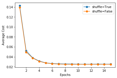
なんだこりゃ! 全く結果は変わりませんね。きっと、一般的には、効果があるのでしょうが、Irisデータセットには合わなかった様ですね。
なるほど、本でもshuffleのオン、オフの違いを載せてないのは、そういうことね。
では、また。