1.はじめに
Python機械学習プログラミング[第2版] という本を買って勉強を始めました。効率的な学習を進める為には、勉強した内容をアウトプットするのが効果的ということで、勉強した内容を備忘録の形でここに残すことを進めています。
なお、本ではコードを一部 jupyter notebook形式で記載しているようですが、ここでは.py形式でも実行できるような形式で記載したいと思います。
今回は、第3章scikit-learnです。
2. パーセプトロン
scikit-learnには、パーセプトロン、ロジスティック回帰、サポートベクトルマシン、決定木、ランダムフォレスト、K近傍法など分類問題を解くための様々なライブラリー存在します。まず、パーセプトロンから見て行きましょう。
パーセプトロンを一々実装せず、scilit-learn のライブラリーから呼び出すだけで済むので便利ですね。
from matplotlib.colors import ListedColormap
import matplotlib.pyplot as plt
from sklearn.metrics import accuracy_score  # sklearn精度表示ライブラリー
import numpy as np

# 決定領域表示関数
def plot_decision_regions(X, y, classifier, test_idx=None, resolution=0.02):

    markers = ('s', 'x', 'o', '^', 'v')
    colors = ('red', 'blue', 'lightgreen', 'gray', 'cyan')
    cmap = ListedColormap(colors[:len(np.unique(y))])

    x1_min, x1_max = X[:, 0].min() - 1, X[:, 0].max() + 1
    x2_min, x2_max = X[:, 1].min() - 1, X[:, 1].max() + 1
    xx1, xx2 = np.meshgrid(np.arange(x1_min, x1_max, resolution),
                           np.arange(x2_min, x2_max, resolution))
    Z = classifier.predict(np.array([xx1.ravel(), xx2.ravel()]).T)
    Z = Z.reshape(xx1.shape)
    plt.contourf(xx1, xx2, Z, alpha=0.3, cmap=cmap)
    plt.xlim(xx1.min(), xx1.max())
    plt.ylim(xx2.min(), xx2.max())

    # 全てのサンプルを表示
    for idx, cl in enumerate(np.unique(y)):
        plt.scatter(x=X[y == cl, 0],
                    y=X[y == cl, 1],
                    alpha=0.8,
                    c=colors[idx],
                    marker=markers[idx],
                    label=cl,
                    edgecolor='black')

    # テストサンプルに丸を付ける
    if test_idx:
        X_test, y_test = X[test_idx, :], y[test_idx]
        plt.scatter(X_test[:, 0],
                    X_test[:, 1],
                    c='',
                    edgecolor='black',
                    alpha=1.0,
                    linewidth=1,
                    marker='o',
                    s=100,
                    label='test set')

    # グラフ表示
    plt.xlabel('petal length [standardized]')
    plt.ylabel('petal width [standardized]')
    plt.legend(loc='upper left')
    plt.tight_layout()
    plt.show()

# irisデータセットの読み込み
from sklearn import datasets
iris = datasets.load_iris()
X = iris.data[:, [2, 3]]
y = iris.target

# データセットの分割(trainとtestに)
from sklearn.model_selection import train_test_split
X_train, X_test, y_train, y_test = train_test_split(
    X, y, test_size=0.3, random_state=1, stratify=y)
print('Class labels:', np.unique(y))
print('Labels counts in y:', np.bincount(y))
print('Labels counts in y_train:', np.bincount(y_train))
print('Labels counts in y_test:', np.bincount(y_test))
print()

# Xデータの標準化
from sklearn.preprocessing import StandardScaler
sc = StandardScaler()
sc.fit(X_train)
X_train_std = sc.transform(X_train)
X_test_std = sc.transform(X_test)
X_combined_std = np.vstack((X_train_std, X_test_std))  # 全体プロット用
y_combined = np.hstack((y_train, y_test))  # 全体プロット用

# Perceptron
from sklearn.linear_model import Perceptron
ppn = Perceptron(max_iter=40, eta0=0.1, random_state=0)
ppn.fit(X_train_std, y_train)
# テストデータによる検証
print('Model: Perceptron')
y_pred = ppn.predict(X_test_std)
print('Misclassified samples: %d' % (y_test != y_pred).sum())  # エラー数
print('Accuracy: %.2f' % accuracy_score(y_test, y_pred))  # 精度
# 決定領域表示
plot_decision_regions(X=X_combined_std, y=y_combined,
                      classifier=ppn, test_idx=range(105, 150))
全体の構成は、テキストと若干変えて、これから何度も出て来るコードは、最初にまとめています。
精度を表示する為のライブラリーのインポート 'from sklearn.metrics import accuracy_score' は冒頭に。
毎回同じフォーマットのグラフを描くことになるので、x軸ラベル、y軸ラベル、凡例などの表示は、決定領域表示関数 plot_decision_regions() に含めています。
動作としては、irisのデータセットを読み込み、xは2列目と3列目の2つを採用、yの区分は3種類(前回は2種類)とし、150個のデータセットを学習7割(35×3=105個)、テスト3割(15×3=45個)に分割して使っています。
Xデータは標準化し、パーセプトロンモデルで105個のデータを使って学習を行い、45個のデータを使って検証し精度を求めています。
インスタンス化するところで、テキストは ppn = Perceptron(n_iter=40, eta0=0.1, random_state=1) となっていますが、このままだとエラーになったり、テキストとの再現性がなかったりしました。どうも、sklearnのバージョンを最新版(0.21.3)にした事が影響した様で、それに対応する為、n_iter → max_iter 、random_state=0 に修正しています。
では、コードを実行してみましょう。
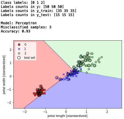
テストデータ45個の内、3個予測を間違えたので、精度は93%(1 - 3/45 = 0.933)です。従って、決定領域の図も上手く分類出来ない結果ですね。
決定領域表示ですが、全データのプロットにテストデータだけ丸を付けるのは、ゴチャゴチャして分かり難い様に思います。それより、テストデータをプロットして、その中で間違えたものだけ丸を付けた方が、分かり易くないでしょうか。ということで、決定領域表示関数を以下の様に改造してみます。
# 決定領域表示関数
def plot_decision_regions(X, y, classifier, test_idx=None, resolution=0.02):

    markers = ('s', 'x', 'o', '^', 'v')
    colors = ('red', 'blue', 'lightgreen', 'gray', 'cyan')
    cmap = ListedColormap(colors[:len(np.unique(y))])

    x1_min, x1_max = X[:, 0].min() - 1, X[:, 0].max() + 1
    x2_min, x2_max = X[:, 1].min() - 1, X[:, 1].max() + 1
    xx1, xx2 = np.meshgrid(np.arange(x1_min, x1_max, resolution),
                           np.arange(x2_min, x2_max, resolution))
    Z = classifier.predict(np.array([xx1.ravel(), xx2.ravel()]).T)
    Z = Z.reshape(xx1.shape)
    plt.contourf(xx1, xx2, Z, alpha=0.3, cmap=cmap)
    plt.xlim(xx1.min(), xx1.max())
    plt.ylim(xx2.min(), xx2.max())

    # テストデータのみプロット(改造)
    for idx, cl in enumerate(np.unique(y)):
        X_test, y_test = X[test_idx, :], y[test_idx]
        plt.scatter(x=X_test[y_test == cl, 0],
                    y=X_test[y_test == cl, 1],
                    alpha=0.8,
                    c=colors[idx],
                    marker=markers[idx],
                    label=cl,
                    edgecolor='black')

    # テストデータでエラーを起こしたものだけ丸を付ける(改造)
    if test_idx:
        X_test, y_test = X[test_idx, :], y[test_idx]
        plt.scatter(X_test[ y_test != y_pred  , 0],
                    X_test[ y_test != y_pred  , 1],
                    c='',
                    edgecolor='black',
                    alpha=1.0,
                    linewidth=1,
                    marker='o',
                    s=100,
                    label='test set')

    # グラフ表示
    plt.xlabel('petal length [standardized]')
    plt.ylabel('petal width [standardized]')
    plt.legend(loc='upper left')
    plt.tight_layout()
    plt.show()
この改造したコードで実行すると、
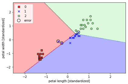
こう表現すると、テストデータ中の「1」の予測を3つ間違えた事が良く分かります。この後は、決定領域表示は、この形で見て行こうと思います。
3.ロジスティック回帰
次に、線形回帰を分類問題に応用したロジスティック回帰です。ロジスティック回帰のアルゴリズムは、
① 対数オッズと呼ばれる値を、重回帰分析により予測する
② 対数オッズをロジット変換(0〜1の間に正則化)し、クラスiに属する確率piの予測値を求める
③ 各クラスに属する確率を計算し、最大確率となるクラスが、データの属するクラスと予測する
では、sklearnのライブラリーで動かしてみましょう。
# ロジスティック回帰
from sklearn.linear_model import LogisticRegression
lr = LogisticRegression(solver='lbfgs', multi_class='auto', C=100.0, random_state=1)
lr.fit(X_train_std, y_train)
# テストデータによる検証
print('Model: LogisticRegression')
y_pred = lr.predict(X_test_std)
print('Misclassified samples: %d' % (y_test != y_pred).sum())  # エラー数
print('Accuracy: %.2f' % accuracy_score(y_test, y_pred))  # 精度
# 決定領域表示
plot_decision_regions(X_combined_std, y_combined,
                      classifier=lr, test_idx=range(105, 150))
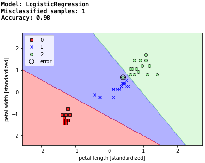
エラー数1、精度98%。 パーセプトロンよりエラー数が減りましたね。
なお、こちらもインスタンス化するところで、テキストのままでは警告が出ましたので、lr = LogisticRegression(C=100.0, random_state=1)を、lr = LogisticRegression(solver='lbfgs', multi_class='auto', C=100.0, random_state=1)
に修正しています。
4.サポートベクトルマシン
次に、マージンの最大化によって分類を行うサポートベクトルマシンです。アルゴリズムを簡単に言えば、分布するデータのど真ん中にピシっと通る直線で分離する、という考え方です。
# サポートベクトルマシン
from sklearn.svm import SVC
svm = SVC(kernel='linear', C=1.0, random_state=1)
svm.fit(X_train_std, y_train)
# テストデータでの検証
print('Model: SVM')
y_pred = svm.predict(X_test_std)
print('Misclassified samples: %d' % (y_test != y_pred).sum())  # エラー数
print('Accuracy: %.2f' % accuracy_score(y_test, y_pred))  # 精度
# 決定領域表示
plot_decision_regions(X_combined_std,
                      y_combined,
                      classifier=svm,
                      test_idx=range(105, 150))
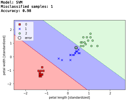
エラー数1、精度98%でした
5.サポートベクトルマシン(カーネルトリック1)
サポートベクトルマシンにカーネル法を適用すると、非線形な解を求める事が出来ます。原理は、カーネル関数を使って、
① データを高次元空間に上手く押し込む
② 高次元空間で線形分離し、その境界線を元の空間に戻す
但し、これをそのまま行うと膨大な計算が必要になる為、カーネルトリックという手法を使って計算量を現実的に抑えつつ計算しています。
# サポートベクトルマシン(カーネルトリック、gamma = 0.2)
svm = SVC(kernel='rbf', random_state=1, gamma=0.2, C=1.0)
svm.fit(X_train_std, y_train)
# テストデータでの検証
print('Model: kernel SVM (gamma = 0.2)')
y_pred = svm.predict(X_test_std)
print('Misclassified samples: %d' % (y_test != y_pred).sum())  # エラー数
print('Accuracy: %.2f' % accuracy_score(y_test, y_pred))  # 精度
# 決定領域表示
plot_decision_regions(X_combined_std, y_combined,
                      classifier=svm, test_idx=range(105, 150))
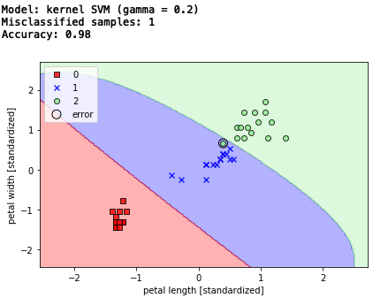
エラー数は変わりませんが、単なる直線的な分離ではなく。なんとなく決定領域がそれらしくなった様な気がしますね。
6. サポートベクトルマシン(カーネルトリック2)
gamma を大きな数字にすると、かなり決定領域を絞り込み、トレーニングデータセットに非常に上手く適合する様になりますが、一方で未知のデータに対しては汎化性は低くなってしまいます。
# サポートベクトルマシン(カーネルトリック、gamma = 100.0)
svm = SVC(kernel='rbf', random_state=1, gamma=100.0, C=1.0)
svm.fit(X_train_std, y_train)
# テストデータでの検証
print('Model: kernel SVM (gamma = 100)')
y_pred = svm.predict(X_test_std)
print('Misclassified samples: %d' % (y_test != y_pred).sum())  # エラー数
print('Accuracy: %.2f' % accuracy_score(y_test, y_pred))  # 精度
# 決定領域表示
plot_decision_regions(X_combined_std, y_combined,
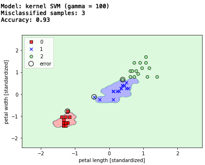
たぶん、トレーニングデータでは、実に上手く決定領域を分けたんでしょうが、テストデータを与えると3個エラーが発生しています。いわゆる、過学習に陥った訳ですね。
7.決定木
一連の質問に基づいて決断を下すことで、データを分類するモデル。アルゴリズムは、情報利得を最大化する分割(分割後のジニ不純度が低いものを優先)をある深さで行い、特徴空間を矩形に分割させます。
ここでは、最大深さ4でトレーニングを行っています。
# 決定木
from sklearn.tree import DecisionTreeClassifier
tree = DecisionTreeClassifier(criterion='gini',
                              max_depth=4,
                              random_state=1)
tree.fit(X_train_std, y_train)  ### +std
# テストデータでの検証
print('Model: Decision Tree')
y_pred = tree.predict(X_test_std)
print('Misclassified samples: %d' % (y_test != y_pred).sum())  # エラー数
print('Accuracy: %.2f' % accuracy_score(y_test, y_pred))  # 精度
# 決定領域表示
plot_decision_regions(X_combined_std, y_combined,
                      classifier=tree, test_idx=range(105, 150))
                      classifier=svm, test_idx=range(105, 150))
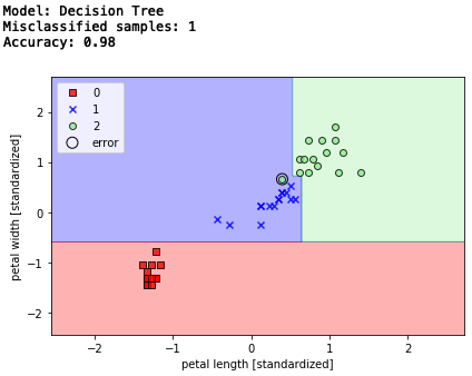
矩形の領域線がいかにも決定木という形ですね。エラー数1、精度98%です。
8.ランダムフォレスト
決定木のアンサンブル版であるランダムフォレストを見てみよう。
アルゴリズムは、データセットからn個のデータ(ブートストラップ標本)をランダムに選択し、そこからランダムにd個のデータを抽出して、決定木を作ることをk回繰り返し、複数のモデルの多数決に基づいてクラスラベルを決定(バギング)するというもの。
通常は、ブートストラップは、トレーニングデータセットのデータ数と同じになっています。
# ランダムフォレスト
from sklearn.ensemble import RandomForestClassifier
forest = RandomForestClassifier(criterion='gini',
                                n_estimators=25,
                                random_state=1,
                                n_jobs=2)
forest.fit(X_train_std, y_train)
#  テストデータでの検証
print('Model: Random Forest')
y_pred = forest.predict(X_test_std)
print('Misclassified samples: %d' % (y_test != y_pred).sum())  # エラー数
print('Accuracy: %.2f' % accuracy_score(y_test, y_pred))  # 精度
# 決定領域表示
plot_decision_regions(X_combined_std, y_combined,
                      classifier=forest, test_idx=range(105, 150))
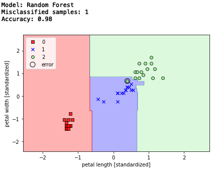
エラー数1,精度98%と変わりませんが、決定木がグレードアップした感じです。
9.K近傍法
最後は、トレーニングデータセットから判別関数を学習する事なく、トレーニングデータセット全部を暗記するモデル、K近傍法です。
アルゴリズムは、トレーニングデータセットの中から予測する点に最も近いk個のデータを見つけ出し、k個のデータの多数決でクラスラベルを決めるというもの。
新しいトレーニングデータを追加する度に、より良いモデルにはなるものの、計算量はそれに比例して増加します。また、大きなデータセットを扱う場合は記憶域が問題になるかもしれません。
ここでは、k = 5 で、行っています。
# K近傍法
from sklearn.neighbors import KNeighborsClassifier
knn = KNeighborsClassifier(n_neighbors=5,
                           p=2,
                           metric='minkowski')
knn.fit(X_train_std, y_train)
# テストデータによる検証
print('Model: KNN')
y_pred = knn.predict(X_test_std)
print('Misclassified samples: %d' % (y_test != y_pred).sum())  # エラー数
print('Accuracy: %.2f' % accuracy_score(y_test, y_pred))  # 精度
# 決定領域表示
plot_decision_regions(X_combined_std, y_combined,
                      classifier=knn, test_idx=range(105, 150))
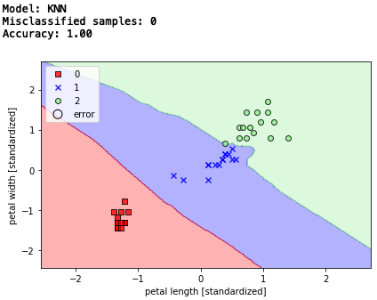
「1」と「2」の混在する部分を上手く切り分けて、精度は100%を達成しました。