深層学習／VAE (Variational Autoencoder) を実装する

1.はじめに

　今回は、Variational Autoencoder を keras で実装してみます。

2.プリミティブなAutoencoder

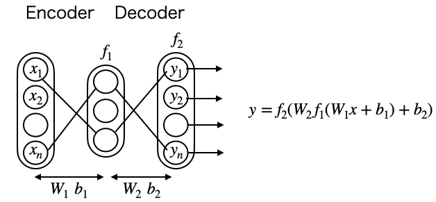
　プリミティブなAutoencoderを考えてみます。入力xに、重みW1とバイアスb1が掛かり活性化関数f1を通して中間層に写像され、さらに重みW2とバイアスb2が掛かり活性化関数f2を通して出力されるとします。

　この時、f2は恒等関数とし、損失関数は二乗誤差の和を取ると、出力yは入力xを再現する様に学習が進みます。W1, b1はデータを表す特徴量と呼ばれます。

3.Autoencoderの実装

　まずは、簡単なオートエンコーダから実装してみます。データセットはMNISTを使います。

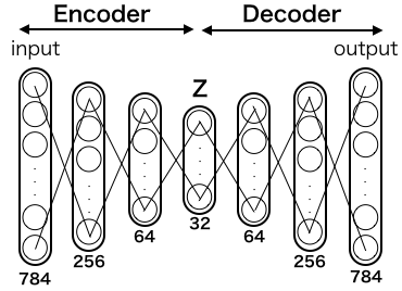
　入力画像は MNIST なので28*28=784次元、それを256次元、64次元、32次元と絞り込んだ後に、64次元、256次元、784次元と元に戻します。損失関数は、出力画像と入力画像の差のクロスエントロピーを取ったものです。

　途中次元数が絞り込まれるため、ニューラルネットワークは、重要な特徴量のみを残そうとして重みを学習します。学習後は input に画像を入れるとそれとほぼ同じ画像を output から出力する様になるわけです。

　では、下記コードを動かしてみます。

from keras.layers import Input, Dense
from keras.models import Model
from keras.datasets import mnist
import numpy as np
import matplotlib.pyplot as plt

# データセット読み込み
(x_train, _), (x_test, _) = mnist.load_data()
x_train = x_train.astype('float32') / 255.
x_test = x_test.astype('float32') / 255.
x_train = x_train.reshape((len(x_train), np.prod(x_train.shape[1:])))
x_test = x_test.reshape((len(x_test), np.prod(x_test.shape[1:])))

# モデル構築
encoding_dim = 32
input_img = Input(shape=(784,))
x1 = Dense(256, activation='relu')(input_img)  
x2 = Dense(64, activation='relu')(x1)  
encoded = Dense(encoding_dim, activation='relu')(x2) 
x3 = Dense(64, activation='relu')(encoded)
x4 = Dense(256, activation='relu')(x3)  
decoded = Dense(784, activation='sigmoid')(x4) 
autoencoder = Model(input=input_img, output=decoded)
autoencoder.compile(optimizer='adadelta', loss='binary_crossentropy')
autoencoder.summary()  

# 学習
autoencoder.fit(x_train, x_train,
                nb_epoch=50,    
                batch_size=256,
                shuffle=True,
                validation_data=(x_test, x_test))

# 学習モデルでテスト画像を変換
decoded_imgs = autoencoder.predict(x_test)

n = 10
plt.figure(figsize=(10, 2))
for i in range(n):
    # テスト画像を表示
    ax = plt.subplot(2, n, i+1)
    plt.imshow(x_test[i].reshape(28, 28))
    plt.gray()
    ax.get_xaxis().set_visible(False)
    ax.get_yaxis().set_visible(False)

    # 変換画像を表示
    ax = plt.subplot(2, n, i+1+n)
    plt.imshow(decoded_imgs[i].reshape(28, 28))
    plt.gray()
    ax.get_xaxis().set_visible(False)
    ax.get_yaxis().set_visible(False)
plt.show()

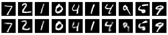
　上段がオリジナルのテスト画像、下段がテスト画像をオートエンコーダで変換した画像です。ほぼほぼテスト画像の再現が出来ていると思います。

　ところで出力は、一番絞り込まれた32次元のZ層の信号によって決まるわけです。言い換えれば32次元の潜在空間Zに様々な形の0〜9の数字が分布していると言えます。

　32次元は、我々は実際に見ることは出来ませんが、グッと次元数を落として潜在空間zを2次元にしたらどうでしょうか。2次元なら、0〜9の数字がどう分布しているか平面に表すことが出来ますからね。

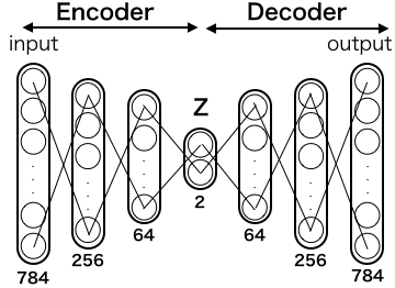
　では、一番絞り込んだ部分を2次元にした場合が、どうなるか見てみましょう。先程のコードのencoding_dim = 32 を encoding_dim = 2に変更して実行すればOKです。

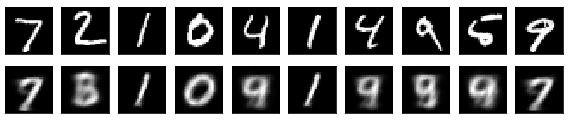
　さすがに潜在空間zが2次元だと再現が難しいですね。「0」,「1」,「7」は再現していますが、残りは他の数字と混じってしまって上手く再現出来ていません。

　言い換えれば、2次元という狭い潜在空間では、0〜9の数字が綺麗に分かれて分布出来ず、多くの数字が混じって分布している様です。

4.VAEモデル

　狭い潜在空間Zの中に、0〜9の数字を重なりなく上手く分布させるには、どうしたら良いでしょうか。自然界の代表的な分布といえば正規分布（ガウス分布）なので、ここでは0〜9の数字の分布は正規分布に従うと仮定して、こんなモデルを考えてみます。

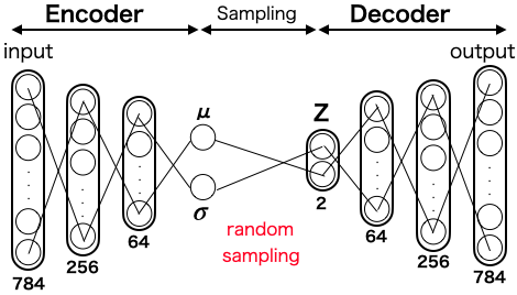
　ある数字がinputに入って64次元まで絞り込まれたら、平均$\mu$ 分散$\sigma$ を調べ、その数字がどんな正規分布に属しているかを求めます。その分布の中からランダムサンプリングした値をZに入れると共に、inputとoutputの差がなくなる様に、Decoderの重みを学習します。こうすることで、0〜9の数字が重なりなく上手く分布させることが出来そうです。

　但し、この考え方には問題点があって、ランダムサンプリングの要素を入れると、誤差逆伝播が出来なくなってしまいます。そこで、この考え方を生かしつつ、誤差逆伝播を可能にしたのが、こんなモデルです。

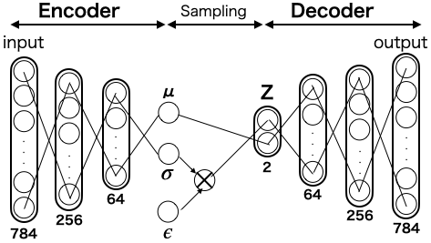
　ここで、$\epsilon$は非常に小さなランダム数です。分散$\sigma$ にこの$\epsilon$を掛けてあげるのです。この手法を Reparametrization Trick と言います。$\mu$=z_mean, $\sigma$=z_logvar, $\epsilon$=epsilonとして、この部分をコード化すると、

# Reparametrization Trick
def sampling(args):
    z_mean, z_logvar = args
    batch = K.shape(z_mean)[0]
    dim = K.int_shape(z_mean)[1]
    epsilon = K.random_normal(shape=(batch, dim)) # ε
    return z_mean + K.exp(0.5 * z_logvar) * epsilon

5.VAEの損失関数

　VAEの損失関数$L$は、以下の様に表わされます。
　　$L =
E_{z \sim q(z|x)}
log_{Pmodel}(x|z) -
D_{KL}(q(z|x)||Pmodel(z))
$

　第1項はq(z|X)に関するデータXの対数尤度の期待値で、出力が元のデータに近いかどうかを表していますので、二乗誤差に置き換えます。第2項は、カルバックライブラー距離($D_{KL}$はKLダイバージェンスを表します)といい、p(z)は正規分布とすると、

　　$=\beta||y-x||^2 - D_{KL}
(N(\mu, \sigma)|N(0,1))\
$

　第2項は kl_loss と表し、$\sigma^2$=z_logvar, $\mu$=z_mean とし、さらに近似式に置き換えると、損失関数$L$(vae_loss)は、下記の様になります。

# 損失関数
# Kullback-Leibler Loss
kl_loss = 1 + z_logvar - K.square(z_mean) - K.exp(z_logvar)
kl_loss = K.sum(kl_loss, axis=-1)
kl_loss *= -0.5

# Reconstruction Loss
reconstruction_loss = mse(inputs, outputs)
reconstruction_loss *= original_dim

vae_loss = K.mean(reconstruction_loss + kl_loss)

6.VAE全体の実装

　先程のコードを含めて、VAE全体のコードを書いて実行してみましょう。

from __future__ import absolute_import
from __future__ import division
from __future__ import print_function
from keras.layers import Lambda, Input, Dense
from keras.models import Model
from keras.datasets import mnist
from keras.losses import mse 
from keras import backend as K
import numpy as np
import matplotlib.pyplot as plt

# データセット読み込み
(x_train, y_train), (x_test, y_test) = mnist.load_data()
image_size = x_train.shape[1] # = 784
original_dim = image_size * image_size
x_train = np.reshape(x_train, [-1, original_dim])
x_test = np.reshape(x_test, [-1, original_dim])
x_train = x_train.astype('float32') / 255
x_test = x_test.astype('float32') / 255

input_shape = (original_dim, )
latent_dim = 2

# Reparametrization Trick 
def sampling(args):
    z_mean, z_logvar = args
    batch = K.shape(z_mean)[0]
    dim = K.int_shape(z_mean)[1]
    epsilon = K.random_normal(shape=(batch, dim), seed = 5) # ε
    return z_mean + K.exp(0.5 * z_logvar) * epsilon

# VAEモデル構築
inputs = Input(shape=input_shape)
x1 = Dense(256, activation='relu')(inputs)  
x2 = Dense(64, activation='relu')(x1) 
z_mean = Dense(latent_dim)(x2)
z_logvar = Dense(latent_dim)(x2)
z = Lambda(sampling, output_shape=(latent_dim,))([z_mean, z_logvar])
encoder = Model(inputs, [z_mean, z_logvar, z], name='encoder')
encoder.summary()

latent_inputs = Input(shape=(latent_dim,))
x3 = Dense(64, activation='relu')(latent_inputs)  
x4 = Dense(256, activation='relu')(x3)  
outputs = Dense(original_dim, activation='sigmoid')(x4)
decoder = Model(latent_inputs, outputs, name='decoder')
decoder.summary()

z_output = encoder(inputs)[2]
outputs = decoder(z_output)
vae = Model(inputs, outputs, name='variational_autoencoder')

# 損失関数
# Kullback-Leibler Loss
kl_loss = 1 + z_logvar - K.square(z_mean) - K.exp(z_logvar)
kl_loss = K.sum(kl_loss, axis=-1)
kl_loss *= -0.5
# Reconstruction Loss
reconstruction_loss = mse(inputs, outputs)
reconstruction_loss *= original_dim

vae_loss = K.mean(reconstruction_loss + kl_loss)
vae.add_loss(vae_loss)
vae.compile(optimizer='adam')
vae.fit(x_train,
                epochs=50,
                batch_size=256,
                validation_data=(x_test, None))

# テスト画像を変換
decoded_imgs = vae.predict(x_test)

# テスト画像と変換画像の表示
n = 10
plt.figure(figsize=(10, 2))
for i in range(n):
    # テスト画像を表示
    ax = plt.subplot(2, n, i+1)
    plt.imshow(x_test[i].reshape(28, 28))
    plt.gray()
    ax.get_xaxis().set_visible(False)
    ax.get_yaxis().set_visible(False)

    # 変換された画像を表示
    ax = plt.subplot(2, n, i+1+n)
    plt.imshow(decoded_imgs[i].reshape(28, 28))
    plt.gray()
    ax.get_xaxis().set_visible(False)
    ax.get_yaxis().set_visible(False)
plt.show()

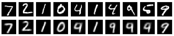
　潜在空間zがたった2次元でも結構再現が出来る様になりました。「0」,「1」,「2」,「7」,「9」と多くの数字が再現出来ています。「4」,「5」は、まだだめですが。

7.潜在空間zを平面で表してみる

　潜在空間Zは2次元ですから平面に表せます。そこに数字の0〜9がどう分布しているか、そこに分布している画像はどんな形なのかを見てみましょう。VAE全体のコードに下記を追加して実行します。

import matplotlib.cm as cm
def plot_results(encoder,
                 decoder,
                 x_test,
                 y_test,
                 batch_size=128,
                 model_name="vae_mnist"):
    z_mean, _, _ = encoder.predict(x_test,
                                   batch_size=128)
    plt.figure(figsize=(12, 10))
    cmap=cm.tab10
    plt.scatter(z_mean[:, 0], z_mean[:, 1], c=cmap(y_test))
    m = cm.ScalarMappable(cmap=cmap)
    m.set_array(y_test)
    plt.colorbar(m)
    plt.xlabel("z[0]")
    plt.ylabel("z[1]")
    plt.show()

    # (-4, -4) から (4, 4) までを30x30分割してプロットする
    n = 30  # 50>30
    digit_size = 28
    figure = np.zeros((digit_size * n, digit_size * n))
    grid_x = np.linspace(-4, 4, n)
    grid_y = np.linspace(-4, 4, n)[::-1]
    for i, yi in enumerate(grid_y):
        for j, xi in enumerate(grid_x):
            z_sample = np.array([[xi, yi]])
            x_decoded = decoder.predict(z_sample)
            digit = x_decoded[0].reshape(digit_size, digit_size)
            figure[i * digit_size: (i + 1) * digit_size,
                   j * digit_size: (j + 1) * digit_size] = digit
    plt.figure(figsize=(10, 10))
    start_range = digit_size // 2
    end_range = n * digit_size + start_range + 1
    pixel_range = np.arange(start_range, end_range, digit_size)
    sample_range_x = np.round(grid_x, 1)
    sample_range_y = np.round(grid_y, 1)
    plt.xticks(pixel_range, sample_range_x)
    plt.yticks(pixel_range, sample_range_y)
    plt.xlabel("z[0]")
    plt.ylabel("z[1]")
    plt.axis('off')
    plt.imshow(figure, cmap='Greys_r')
    #plt.savefig(filename)
    plt.show()

plot_results(encoder,
                 decoder,
                 x_test,
                 y_test,
                 batch_size=128,
                 model_name="vae_mlp")

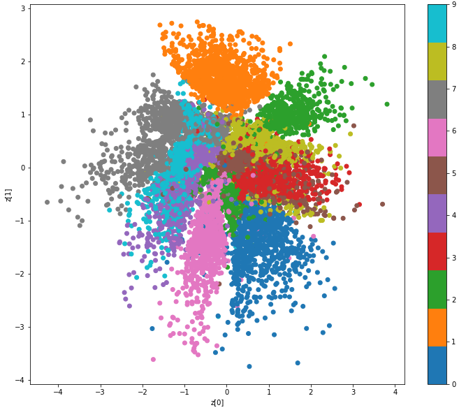
　「0」,「1」,「2」,「6」,「7」は他の数字との重なりがなく分布している様です。

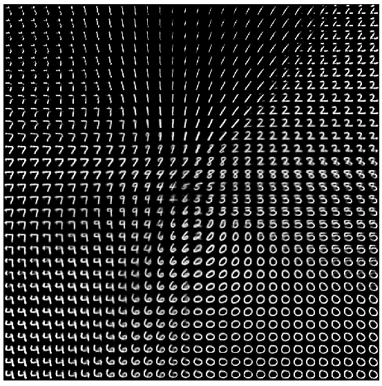
　正規分布に沿って分布させているので、ある数字からある数字へ連続的に変化していることが分かります。