はじめに
スモールデータと機械学習より、線形判別分析 (LDA) の理解を深めるために記事を作成します。n番煎じです。この記事では基本的にベクトルは縦ベクトルとして扱います。
ついでに LDA の考え方を活用した事例として、腸内細菌叢の研究で用いられる LEfSe、画像処理の二値化で用いられれる大津の二値化の処理内容も出力します。
LDA の概要
- 分類問題に使われるアルゴリズム(下図は明治大金子先生の HP から一部借用)
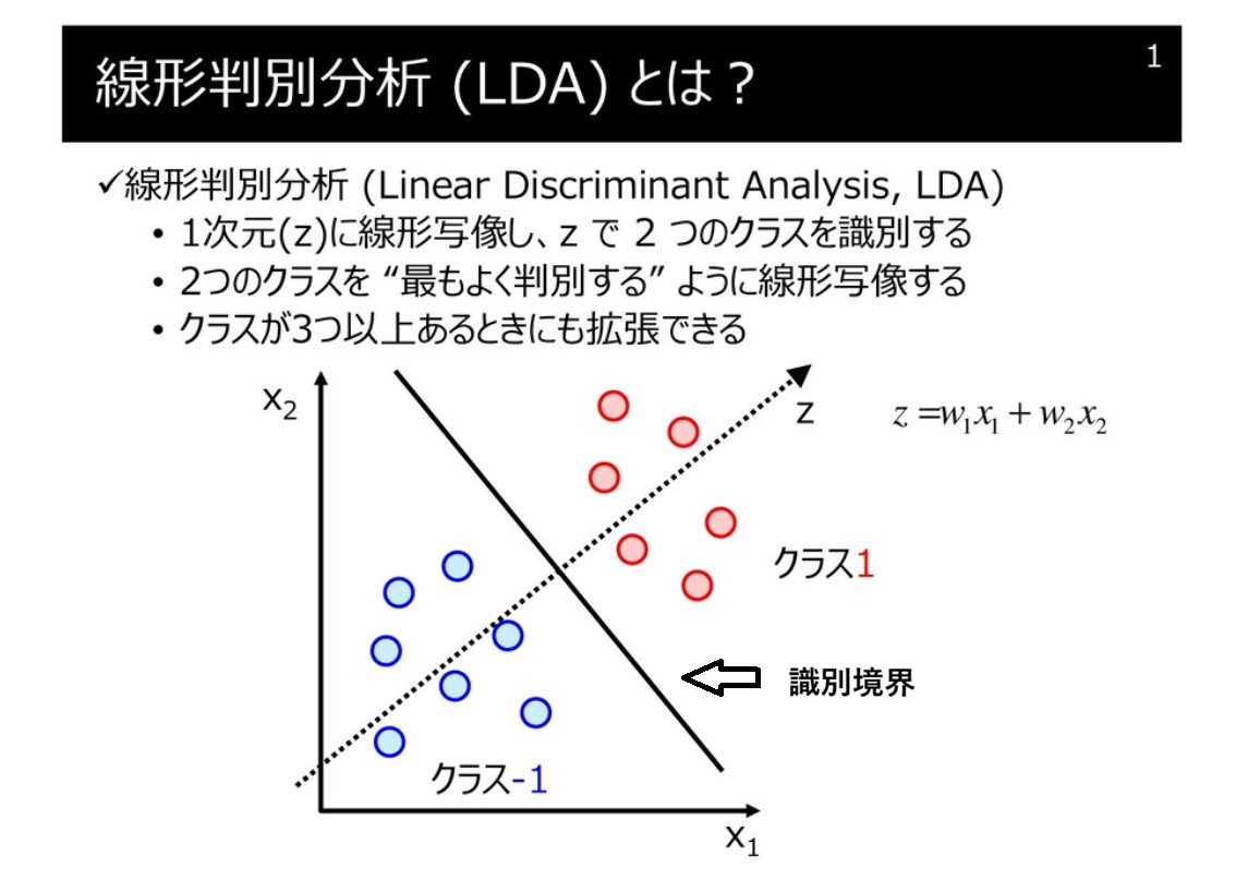
- 分類に際し、クラスの平均ベクトル間の距離が最大に、クラス内の分散が最小になるような変換を行う方向ベクトル $w$ を求める
導出
データセット ($X, X \in \mathbb{R}^{N \times M}$, $N$: データ数, $M$: 説明変数の次元) 、およびそれに対応する分類クラス ($C_1, C_2$) があります。クラスの分離度 (クラスの平均ベクトル間の距離) が最大になる、かつ、クラス内の分散が最小になる識別境界を引くことができれば、よくクラスを識別することができそうです。
クラス $C_1, C_2$ の平均ベクトル $m_1, m_2$ を計算します。$N_1, N_2$ は $C_1, C_2$ のサンプル数です。
\begin{align}
m_1 = \frac{1}{N_1} \sum_{n \in C_1} x_n \\
m_2 = \frac{1}{N_2} \sum_{n \in C_2} x_n
\end{align}
$m_1, m_2$ 間の距離が最大になるような方向ベクトル $w$ ($||w|| = 1$) を与えます。
w^\mathsf{T} m_1 - w^\mathsf{T} m_2 = w^\mathsf{T} (m_1 - m_2)
次に $w$ で一次元に変換した後の $C_1, C_2$ のクラス内分散 $s_1, s_2$ を考えます。
\begin{align}
s_1 &= \sum_{n \in C_1} (w^\mathsf{T} x_n - w^\mathsf{T} m_1)^2 \\
s_2 &= \sum_{n \in C_2} (w^\mathsf{T} x_n - w^\mathsf{T} m_2)^2 \\
s &= s_1 + s_2
\end{align}
クラス間分散を分子に、クラス内変動を分母にとる関数 $J(w)$ を最大化する方向ベクトル $w$ を探索します。
\begin{align}
J(w)&= \frac{w^\mathsf{T} S_B w}{w^\mathsf{T} S_W w} \\
S_B &= (m_1 - m_2)(m_1 - m_2)^\mathsf{T} \\
S_W &= \sum_{n \in C_1}  (x_n -  m_1)(x_n - m_1)^\mathsf{T} + \sum_{n \in C_2}  (x_n -  m_2)(x_n - m_2)^\mathsf{T}
\end{align}
極値を探すため、$J(w)$ を微分し、$0$ とおきます。
\begin{align}
\frac{\delta J(w)}{\delta w}
&= \frac{(w^\mathsf{T} S_B w)'(w^\mathsf{T} S_W w) - (w^\mathsf{T} S_B w)(w^\mathsf{T} S_W w)'}{(w^\mathsf{T} S_W w)^2} \\
&= \frac{2 S_B w w^\mathsf{T} S_w w -2 w^\mathsf{T} S_B w S_w w}{(w^\mathsf{T} S_W w)^2} \\
&= 0 \\
\end{align}
$w^\mathsf{T} S_B w$ および $w^\mathsf{T} S_W w$ の計算結果はスカラーなので、順序を入れかえて式を整理します。その後、両辺を $w^\mathsf{T} S_W w$ で除します。
\begin{align}
(w^\mathsf{T} S_W w)S_B w &=  (w^\mathsf{T} S_B w)S_W w \\
S_B w &= \frac{w^\mathsf{T} S_B w}{w^\mathsf{T} S_W w} S_W w
\end{align}
定数 $\lambda = \frac{w^\mathsf{T} S_B w}{w^\mathsf{T} S_W w}$ とおくと
\begin{align}
S_B w = \lambda S_W w \\
\underbrace{S_W^{-1}}_{S_W の逆行列を左からかける} S_B w = \lambda w
\end{align}
となり、固有値問題として解くことで、固有値 $\lambda = \frac{w^\mathsf{T} S_B w}{w^\mathsf{T} S_W w}$ が最大の時の固有ベクトル $w$ をもとめることができます。
実装
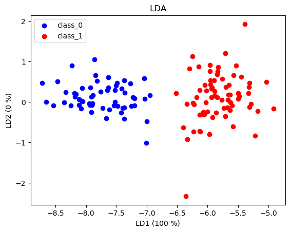
sklearn のwine_datasetは 3 種類の異なる品種から作られたワインの化学分析結果をまとめたデータセットです。このデータセットのclass_0 class_1 をLDAで分類してみます。ついでに、主成分分析の各主成分軸の寄与率のように、各固有値の占める割合を軸に書き加えてみます。
- wine dataset

import numpy as np
import pandas as pd
import matplotlib.pyplot as plt
from sklearn.datasets import load_wine
from sklearn.discriminant_analysis import LinearDiscriminantAnalysis

wine = load_wine()
data = wine.data
target = wine.target
columns = wine.feature_names


df_wine = pd.DataFrame(data, columns=columns)
df_wine["target"] = target
df_0 = df_wine[df_wine["target"]==0]
df_1 = df_wine[df_wine["target"]==1]
x_0 = np.array(df_0.iloc[:, :-1])
x_1 = np.array(df_1.iloc[:, :-1])
labels = np.unique(target)
def LDA_2class(a, b, label):

    m_a, m_b = a.mean(axis=0).reshape(-1,1), b.mean(axis=0).reshape(-1,1)
    # S_B
    s_b =  np.outer((m_a - m_b), (m_a - m_b))
    list_ab = [a, b]
    list_m = [m_a, m_b]

    # S_w
    s_w = np.zeros((a.shape[1], a.shape[1]))
    for c, m in zip(list_ab, list_m):
        for i in range(a.shape[0]):
            s_w += np.outer((c[i, :].reshape(-1, 1) - m), (c[i, :].reshape(-1, 1) - m))

    # solving an eigen value problem
    eig_vals, eig_vecs = np.linalg.eig(np.linalg.inv(s_w) @(s_b))

    idx = np.argsort(eig_vals)[::-1]
    eig_vals_sorted = eig_vals[idx]
    eig_vecs_sorted = eig_vecs[:, idx]

    eig_vals_ratio = eig_vals_sorted.real / eig_vals_sorted.real.sum()

    w1a = a @ eig_vecs_sorted[:, :2]
    w1b = b @ eig_vecs_sorted[:, :2]
    plt.scatter(w1a[:, 0], w1a[:, 1], color='blue', label=f'class_{label[0]}')
    plt.scatter(w1b[:, 0], w1b[:, 1], color='red', label=f'class_{label[1]}')
    plt.title('LDA')
    plt.xlabel(f'LD1 ({round(eig_vals_ratio[0]*100)} %)')
    plt.ylabel(f'LD2 ({round(eig_vals_ratio[1]*100)} %)')
    plt.legend()
    plt.show()

LDA_2class(x_0, x_1, labels[:2])
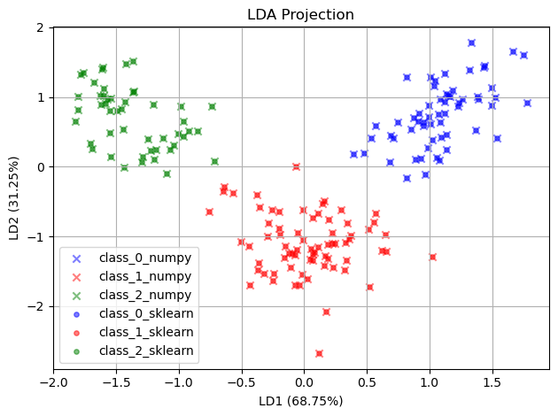
3 クラス以上の LDA の計算をchatGPT に出力させてみると、以下のコードが sklearn.discriminant_analysis.LinearDiscriminantAnalysis の結果と重なりました。どうやらクラス間分散 $S_B$ の計算に全てのクラスの平均を用いているようです。
# ----- 1) データ読み込み(例として Iris データセットを使用) -----
X, y = wine.data, wine.target
classes = np.unique(y)
target_names_numpy = [name + '_numpy' for name in wine.target_names]
target_names_sklearn = [name + '_sklearn' for name in wine.target_names]

# ----- 2) SW, SB の計算 -----
def compute_sw_sb(X, y):
    n_features = X.shape[1]
    overall_mean = np.mean(X, axis=0)
    SW = np.zeros((n_features, n_features))
    SB = np.zeros((n_features, n_features))

    for c in classes:
        Xc = X[y == c]
        mean_c = np.mean(Xc, axis=0)
        # クラス内散布
        SW += (Xc - mean_c).T @ (Xc - mean_c)
        # クラス間散布
        n_c = Xc.shape[0]
        mean_diff = (mean_c - overall_mean).reshape(n_features, 1)
        SB += n_c * (mean_diff @ mean_diff.T)
    return SW, SB

SW, SB = compute_sw_sb(X, y)

# ----- 3) 一般化固有値問題の解法 -----
eigvals, eigvecs = np.linalg.eig(np.linalg.inv(SW) @ SB)
# 固有値の大きい順に並び替え
idx = np.argsort(eigvals)[::-1]
W = eigvecs[:, idx[:2]]  # 上位2成分を選択
eigvals_ratio = eigvals[idx[:2]].real / eigvals[idx[:2]].real.sum()

# ----- 4) データを2次元に射影 -----
X_r2 = -X @ W  # (n_samples, 2)
X_r2 = (X_r2 - X_r2.mean(axis=0)) / X_r2.std(axis=0)  # 標準化
# ----- 5) 可視化 -----
colors = [ 'blue', 'red', 'green']
for c, color in zip(classes, colors):
    plt.scatter(X_r2[y == c, 0], X_r2[y == c, 1],
                color=color, label=target_names_numpy[c], alpha=0.5, marker="x")

# LDA で 2 次元射影
lda = LinearDiscriminantAnalysis(n_components=2)
X2 = lda.fit_transform(X, y)
X2 = (X2 - X2.mean(axis=0)) / X2.std(axis=0)  # 標準化
# 散布図を描く
for cls, color, label in zip([0,1,2], ['blue','red','green'], target_names_sklearn):
    plt.scatter(X2[y==cls,0], X2[y==cls,1],
                alpha=0.5, color=color, label=label, marker = "o", s=15)

plt.title('LDA Projection')
plt.xlabel(f'LD1 ({eigvals_ratio[0]*100:.2f}%)')
plt.ylabel(f'LD2 ({eigvals_ratio[1]*100:.2f}%)')
plt.legend(loc='best')#
plt.grid(True)
plt.tight_layout()
plt.show()
LDA の活用事例
LEfSe
LefSe は腸内細菌叢や代謝物などの多変量データに対して、各クラスに特徴的な説明変数を抽出する方法です。Kruskal Wallis 検定でクラス間に差があるかを評価し、Wilcoxon の順位和検定でどの特徴量間に差があるのかを評価し、有意な差に関してLDAで効果量を算出します。LDAの効果量は最も分離する $w_1$ を絶対値に変換し、$w_1$ 内の最小の要素を $1$ に、最大の要素を $10^6$ にスケーリングしたのち、常用対数に変換して得られます。この効果量の算出には $30$ 回のブートストラップサンプリングを行い、平均値を用います。よく腸内細菌叢のデータは占有率で示されるため、定数和制約(特定の菌が多くなるとほかの菌の占有率が下がる)が存在します。LDA はデータに正規分布の性質や変数の独立性を仮定しますが、この時、定数和制約が邪魔になります。そのため、CLR (centerd log-ratio) 変換 などの行ってユークリッド空間上にマッピングしてから LEfSE を行うほうが望ましいかもしれません。$D$ 次元の説明変数 ($ x_1 \cdots x_i \cdots x_d$) に対して、CLR 変換後の説明変数 ($ y_1 \cdots y_i \cdots y_d$) は以下のようにあらわせます。
\begin{align}
y_i
&=  \mathrm{clr}(x_i) \\
&=\ln\frac{x_i}{(\prod_{j=1}^{D} x_{j})^{1/D}}
\end{align}

大津の二値化
概要
大津の二値化は画像を二値化する際に使用される方法のひとつで、二値化に必要な閾値を自動的に決定します。
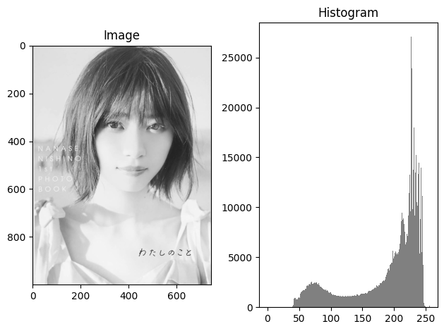
画像ヒストグラムにおいて閾値を決め、閾値未満または閾値以上で画素を2クラスに分けます。クラス間分散とクラス内分散の比を最大化する閾値を探索することで、適切な閾値を設定します。閾値未満をクラス1、閾値以上をクラス2、クラス1、2 の画素数 ($n$) をそれぞれ $n_1, n_2$、クラス1、2の画素値の平均 ($m$)、分散 ($\sigma$)を $m_1, m_2, \sigma_1^2, \sigma_2^2$ とするとクラス間分散 ($S_B$) 、クラス内分散 ($S_W$) は以下の式で表せます。
\begin{align}
S_B
&= \frac{n_1 n_2 (m_1 - m_2)^2}{(n_1 + n_2)^2} \\
S_W
&= \frac{n_1 \sigma_1^2 + n_2 \sigma_2^2}{n_1 + n_2}
\end{align}
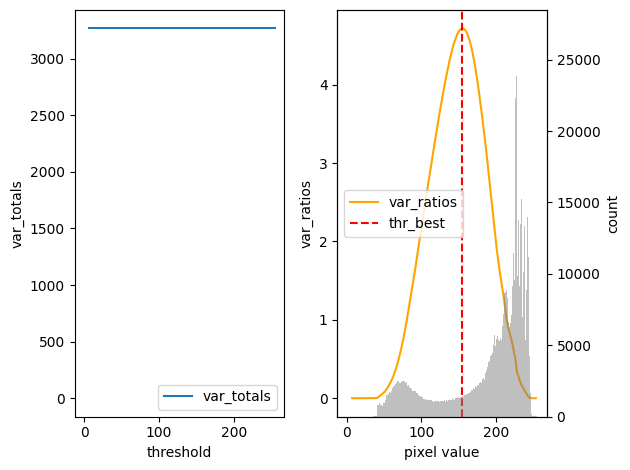
グレースケール画像の画素値は $0-255$ の値をとるため、その範囲の中で最も $\frac{S_B}{S_W}$ が大きい値を示す時の閾値を採用して画像を二値化します。なお、全分散 $\sigma_t^2$ は $S_B + S_W$ となり、一定の値を示します。
参考文献
実装
大津の二値化をnumpy で実装し、OpenCV との結果と比較します。
import numpy as np
import matplotlib.pyplot as plt
import cv2

path_image = r"path_to_image"
img = cv2.imread(path_image, cv2.IMREAD_GRAYSCALE)
fig, ax = plt.subplots(1,2, tight_layout=True)
ax[0].imshow(img, cmap='gray')
ax[1].hist(img.flatten(), bins=256, range=(0, 256), alpha=1, color='gray')
ax[0].set_title('Image')
ax[1].set_title('Histogram')
plt.show()
hist, _ = np.histogram(img.flatten(), bins=256, range=(0, 256))
pixel_value = np.arange(256)
hist_by_value = hist * pixel_value
var_totals = np.zeros(255)
var_ratios = np.zeros(255)
thr_best = 0


for thr in range(1, 255):
    w1 = np.sum(hist[:thr])
    w2 = np.sum(hist[thr:])
    m1 = np.sum(hist_by_value[:thr]) / w1
    m2 = np.sum(hist_by_value[thr:]) / w2
    var1 = np.sum((pixel_value[:thr] - m1) ** 2 * hist[:thr]) / w1
    var2 = np.sum((pixel_value[thr:] - m2) ** 2 * hist[thr:]) / w2
    var_within = (var1 * w1 + var2 * w2) / (w1 + w2)
    var_inter = (m1 - m2) ** 2 * w1 * w2 / (w1 + w2)**2
    var_total = var_within + var_inter
    var_ratio = var_inter / var_within
    if var_ratio >= var_ratios[thr_best]:
        thr_best = thr
    var_ratios[thr] = var_ratio
    var_totals[thr] = var_total
fig_1, ax_1 = plt.subplots(1,2,  tight_layout=True)
ax_1[0].plot(var_totals, label="var_totals")
ax_1[0].set_ylabel("var_totals")
ax_1[0].set_xlabel('threshold')
ax_1[1].plot(var_ratios, label="var_ratios", color='orange')
ax_1[1].set_ylabel("var_ratios")
ax_1_r = ax_1[1].twinx()
ax_1_r.hist(img.flatten(), bins=256, range=(0, 256), alpha=0.5, color='gray')
ax_1_r.set_ylabel("count")
ax_1[1].set_xlabel('pixel value')
ax_1[1].axvline(thr_best, color='red', linestyle='--', label='thr_best')
ax_1[0].legend()
ax_1[1].legend()
plt.show()
thr_value, img_binary = cv2.threshold(img, thr_best, 255, cv2.THRESH_BINARY)
thr_otsu, img_binary_otsu = cv2.threshold(img, 0, 255, cv2.THRESH_BINARY + cv2.THRESH_OTSU)
fig, ax = plt.subplots(1,2,  tight_layout=True)
ax[0].imshow(img_binary, cmap='gray')
ax[0].set_title(f"binary image_numpy, thr = {thr_best}")

ax[1].imshow(img_binary_otsu, cmap='gray')
ax[1].set_title(f"binary image_cv2, thr = {thr_otsu}")
plt.show()
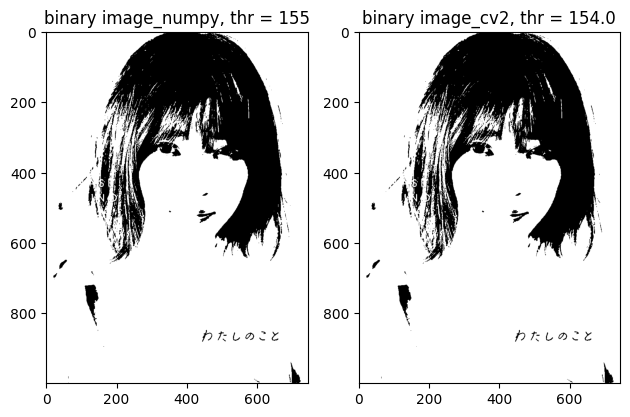
閾値探索は問題なさそうです。
おわりに
線形判別分析を理解するために、自身の学びを出力しました。違っている点など見つかれば適宜修正します。ご指摘いただけると感謝です