はじめに
学習のアウトプットの一環として本記事を投稿します。
投稿内容としては猫と犬の判別ツールを一般開示されているものから抽出し
その精度課題を把握したうえで精度改良のうえ結果を可視化し、その考察を
行ったものです。
目的
画像判別の精度向上
実行環境
Python3
windows10
Chrome
Kaggle Notebook
ステップ(目次)
・公開されている画像判別で精度が低いものをピックアップ
・現状の精度確認
・改良の方向性案を検討
・コード変更による改良
・転移学習を利用した改良
・サンプル評価
・学習結果の可視化(loss, accuracyのエポックごとの推移)
・考察
公開されている画像判別で精度が低いものをピックアップ
犬猫画像の準備
犬か猫かをAIに判別用として事前にモデルに学習させるために、ある程度多くの画像データを
用意する必要があります。今回の画像認識モデルを改良するにあたって、kaggleで公開されて
いるデータセットおよびコードを利用しました。
https://www.kaggle.com/bhrugeshjadav/deep-learning-cnn
# This Python 3 environment comes with many helpful analytics libraries installed
# It is defined by the kaggle/python Docker image: https://github.com/kaggle/docker-python
# For example, here's several helpful packages to load
import numpy as np # linear algebra
import pandas as pd # data processing, CSV file I/O (e.g. pd.read_csv)
# Input data files are available in the read-only "../input/" directory
# For example, running this (by clicking run or pressing Shift+Enter) will list all files under the input directory
import os
for dirname, _, filenames in os.walk('/kaggle/input'):
    for filename in filenames:
        #print(os.path.join(dirname, filename))
        pass
# You can write up to 20GB to the current directory (/kaggle/working/) that gets preserved as output when you create a version using "Save & Run All"
# You can also write temporary files to /kaggle/temp/, but they won't be saved outside of the current session
!pip install imutils
import numpy as np
# import pandas as pd
import tensorflow as tf
import cv2
# import os
from imutils import paths
path = list(paths.list_images("../input/cat-and-dog/training_set/training_set"))
import cv2
path[1]
len(path)
path[1].split("/")
(cv2.imread(path[3])).shape
X_data = []
Y_labels = []
y_data = ['cats','dogs']
for i in range(0,len(path)):
    label = path[i].split("/")[-2]
    if label not in y_data:
        continue
    else:
        image = cv2.imread(path[i])#IMAGE WILL BE SAVED IN ARRAY FORMAT
        image = cv2.cvtColor(image, cv2.COLOR_BGR2RGB)#CONVERT ING INTO RGB FORMAT
        image = cv2.resize(image, (124,124))#APPLY FIX SIZE TO ALL IMAGES
        X_data.append(image)
        Y_labels.append(label)
x_array = np.array(X_data)
y_array = np.array(Y_labels)
x_array.shape,y_array.shape
import matplotlib.pyplot as plt
%matplotlib inline
plt.imshow(x_array[999])
from sklearn.preprocessing import LabelEncoder
from sklearn.model_selection import train_test_split
LE = LabelEncoder()
LE.fit(y_array)
Y_Encoded = LE.transform(y_array)
x_train, x_test, y_train, y_test = train_test_split(x_array, Y_Encoded, test_size = 0.2,random_state=42)
x_train.shape, x_test.shape, y_train.shape, y_test.shape
x_train_norm = x_train/255.
x_test_norm = x_test/255.
model=tf.keras.Sequential()
model.add(tf.keras.layers.Conv2D(32, kernel_size=(3,3),input_shape=(124,124,3),activation='relu'))
model.add(tf.keras.layers.Conv2D(64, kernel_size=(3,3), activation='relu'))
model.add(tf.keras.layers.BatchNormalization())
model.add(tf.keras.layers.MaxPool2D(pool_size=(2,2)))
# Flatten the output
model.add(tf.keras.layers.Flatten())
# Dense layer
model.add(tf.keras.layers.Dense(500, activation='relu'))
model.add(tf.keras.layers.Dense(200, activation='relu'))
model.add(tf.keras.layers.Dense(100, activation='relu'))
model.add(tf.keras.layers.Dense(60, activation='relu'))
model.add(tf.keras.layers.Dense(30, activation='relu'))
# Output layer
model.add(tf.keras.layers.Dense(1, activation='sigmoid'))
model.compile(optimizer='Adam',
              loss='binary_crossentropy', metrics=['accuracy'])
model.fit(x_train_norm,y_train,
          validation_data=(x_test_norm,y_test),
          epochs=7)
現状の精度確認
TRAINING_ACCURACYは高いが、TESTING_ACCURACYは低くEpoch3/7以降は精度が上がっていない。
Epoch 1/7
2022-01-28 21:50:43.579337: I tensorflow/stream_executor/cuda/cuda_dnn.cc:369] Loaded cuDNN version 8005
201/201 [==============================] - 14s 37ms/step - loss: 0.7290 - accuracy: 0.5957 - val_loss: 0.6936 - val_accuracy: 0.5109
Epoch 2/7
201/201 [==============================] - 6s 31ms/step - loss: 0.5903 - accuracy: 0.6866 - val_loss: 0.6447 - val_accuracy: 0.6290
Epoch 3/7
201/201 [==============================] - 6s 32ms/step - loss: 0.4311 - accuracy: 0.8040 - val_loss: 0.6383 - val_accuracy: 0.6908
Epoch 4/7
201/201 [==============================] - 6s 31ms/step - loss: 0.1967 - accuracy: 0.9272 - val_loss: 0.9978 - val_accuracy: 0.6683
Epoch 5/7
201/201 [==================は===========] - 6s 31ms/step - loss: 0.0684 - accuracy: 0.9767 - val_loss: 1.4370 - val_accuracy: 0.6790
Epoch 6/7
201/201 [==============================] - 6s 32ms/step - loss: 0.0547 - accuracy: 0.9825 - val_loss: 1.3004 - val_accuracy: 0.6983
Epoch 7/7
201/201 [==============================] - 6s 31ms/step - loss: 0.0342 - accuracy: 0.9906 - val_loss: 1.3421 - val_accuracy: 0.6746


この画像結果から、過学習が進み汎化性能が高まっていない課題が確認できた。
改良の方向性案を検討
<1>テストサイズの変更
<2>softmaxへの変更
<3>上記で改良が見込めない場合は別の方法を検討
コード変更による改良
<1>テストサイズを0.2から0.3に変更 ⇒ 結果は改良されず
テストサイズを0.2から0.1に変更 ⇒ 結果は改良されず
<2>softmaxへの変更 ⇒ 結果は改良されず、逆に悪化
コード変更で改良が見込まれないため転移学習を活用することとする。
転移学習を利用した改良
VGG16の転移学習を活用した結果、大幅に精度を向上することができた。
input_tensor = Input(shape=(124, 124, 3))
vgg16 = VGG16(include_top=False, weights='imagenet', input_tensor=input_tensor)
top_model = Sequential()
top_model.add(Flatten(input_shape=vgg16.output_shape[1:]))
top_model.add(Dense(256, activation='relu'))
top_model.add(Dropout(0.5))
top_model.add(Dense(1, activation='sigmoid'))
model =Model(inputs=vgg16.input, outputs=top_model(vgg16.output))
for layer in model.layers[:15]:
    layer.trainable =False
from tensorflow.keras.optimizers import Adam
model.summary()
model.compile(loss='binary_crossentropy',
              optimizer=optimizers.Adam(lr=1e-4),
              metrics=['accuracy'])
model.fit(x_train, y_train, validation_data=(x_test, y_test), batch_size=32, epochs=7)
``転移

# サンプル評価
10個のサンプル評価でも十分な精度が確認できた。
predictions = model.predict(x_test).astype(int)
predictions2 = pd.DataFrame(predictions, columns=["Predict"])
y_test2 = pd.DataFrame(y_test, columns=["test"])
compare = pd.concat([predictions2, y_test2], axis=1)
compare.tail(10)
Predict test
1591 0 0
1592 0 0
1593 1 1
1594 0 0
1595 1 1
1596 0 0
1597 0 1
1598 0 0
1599 1 1
1600 0 0
# 学習結果の可視化(loss, accuracyのエポックごとの推移)
history = model.fit(x_train_norm,y_train,
validation_data=(x_test_norm,y_test),
epochs=7)
epochs = 7
fig, (ax1, ax2) = plt.subplots(2, 1, figsize=(12, 12))
ax1.plot(history.history['loss'], color='b', label="Training loss")
ax1.plot(history.history['val_loss'], color='r', label="validation loss")
ax1.set_xticks(np.arange(1, epochs, 1))
ax1.set_yticks(np.arange(0, 1, 0.1))
ax2.plot(history.history['accuracy'], color='b', label="Training accuracy")
ax2.plot(history.history['val_accuracy'], color='r',label="Validation accuracy")
ax2.set_xticks(np.arange(1, epochs, 1))
legend = plt.legend(loc='best', shadow=True)
plt.tight_layout()
plt.show()

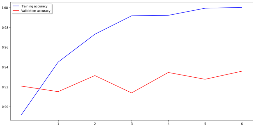
# 考察
転移学習を用いた結果、精度が高まり汎化性能も向上した。改良前のシンプルな学習モデルとは異なり、効果的な仮説を効率的に見つけ出すために、別のタスクで学習された知識を転移する機械学習の手法となる転移学習を用いることで、過学習を防ぎ、汎化性能を高めることができたと推察される。複数の畳み込み層、プーリング層、活性化関数の組み合わせとドロップアウト層からなる学習モデルの開発により生み出されたVGG16の威力を垣間見ることができた。