Zero-Less Decision Diagrams in Dogelog Player

Last updated at 2025-02-06Posted at 2025-02-06

Among algebraic approaches to propositional logic we find binary decision diagrams. The approach is syntactical and not semantical, since it focuses on a certain formulas to represent truth tables. Unlike matrix like disjunctive or conjunctive normal forms, they give tree like normal forms.

Graphic: George Boole

When we first encountered Zero-Suppressed Decision Diagrams (ZDD) we had a hard time implementing all the operations. And accidentally we discovered Zero-Less Decision Diagrams (LDD). Since ZDD have O(2^n) complexity negation operation and LDD only O(1) complexity negation operation, we did some excavation and reengineering.

Binary Decision Diagrams

We start with an introduction to Binary Decision Diagrams (BDD). They were already invented by George Boole in 1854, but are sometimes attribute to a Claude Shannon paper from 1949. Boole's expansion theorem states that every boolean function F can be expanded versus a variable into F = X*F_1 + (1-X)*F_0, were F_1 and F_0 are the cofactors.

A modern reading sees an if-then-else, namely the expansion can be expressed as F = if X then F_1 else F_0. We use the Prolog term (X -> F_1; F_0) to represent such an if-then-else. In the following we do not address issues of common subexpression sharing or caching of operations, which are often seen part and parcel of BDDs.

We can readily present the negation operation and make our point, that it has complexity O(2^n) where n are the number of if-then-else levels. To apply the negate operation to an if-then-else we have to recursively decend and compute two new negate operation, making it exponential.

tree_not(1, 0).
tree_not(0, 1).
tree_not((X->A;B), (X->C;D)) :-
   tree_not(A, C),
   tree_not(B, D).

We use the Prolog lexical ordering (<@)/2 on the variables and assume the input trees are ordered and do produce an ordered output tree as well. The realization of the binary operation requires also a rebuilding of the output tree, where we take the opportunity to reduce the output tree. The result are so called reduced ordered binary decision diagrams (ROBDD):

tree_make(_, A, A, A) :- !.
tree_make(X, A, B, (X->A;B)).

Leaf Property

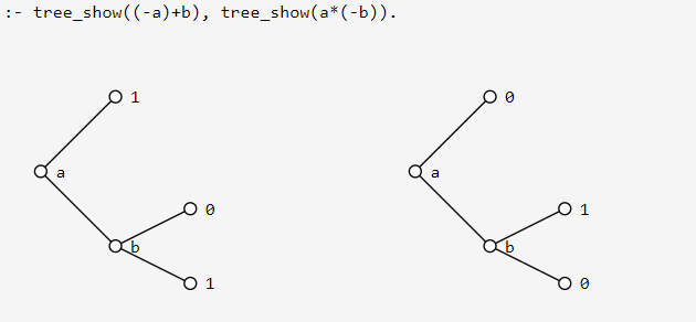
Using our library(vector) we can render the binary decision diagrams inside a Dogelog Notebook. The main routine just traverses the Prolog term and emits SVG drawing drawing commands. Coloring is done in a CSS style sheet, each drawing command refers to one or more CSS class.

Our predicate svg_begin/1 will create a 500x400 coordinates SVG element. We scale it by 50% x 50% so that we later can place multiple SVG elements side by side. We see the leaf property, namely that in our modelling of binary decision diagrams the propositional logic is mainly stored in the leafs:

Zero-Less Decision Diagram

We now turn our attention to Zero-Less Decision Diagrams. In this setting we are still ticking along with Booles expansion represented as (X -> F_1; F_0), but additionally allow also nodes in the tree of the form (- F) that negate a branch. We ban the constant zero 0, it has to be represented by the negated constant one 1, i.e. (- 1).

Since we have negated branches we can use this to turn the negation operation into a one shot operation. There is no more need to recursively decend if-then-else branches. As a result the negation operation has now O(1) complexity:

tree5_not((- A), A) :- !.
tree5_not(A, (- A)).

Again we assume the input trees are ordered and do produce an ordered output tree. Moreover during rebuilding we take again the opportunity to create a unique normal form. This time the rules eliminate certain patterns by shifting the negation to the root.

tree5_make(_, A, A, A) :- !.
tree5_make(X, (-A), (-B), (- (X->A;B))) :- !.
tree5_make(X, (-A), B, (- (X->A; (- B)))) :- !.
tree5_make(X, A, B, (X->A;B)).

Node Property

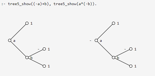
Again using our library(vector) we can render the zero-less decision diagrams inside a Dogelog Notebook. The main routine has to traverse an additional node type of negated branches. Otherwise we proceed similarly as for binary decision diagrams emitting SVG drawings and using CSS classes.

The resulting tree display illustrates possibly best why we call this variant of decision diagrams zero-less. All the leafs have now the value of the constant one 1. The propositional logic is mainly stored in the nodes. An odd number of negations along a branch gives the constant zero 0.

Conclusions

Donald Knuth also popularized zero-suppressed decision diagrams, a binary decision diagram variant developed by Shin-Ichi Minato. Their appeal results from "jump" where nodes are omitted. We focused more on the cost of negation and arrived at zero-less decision diagram. They might have different niche application areas.