この記事はElastic Stack (Elasticsearch) Advent Calendar 2019の19日目の記事です。
はじめに
Vega/Bison/Balrogの日英表記での対応が一生覚えられません。j-yamaです。
某日、某所にて。こんな質問を受けました。
『Kibanaでウォーターフォールチャートって表示できません?エクセルとかにあるやつなんですが。』
(もともとのKibanaにはないけれどVegaのExampleにはあったような…探してみよう)
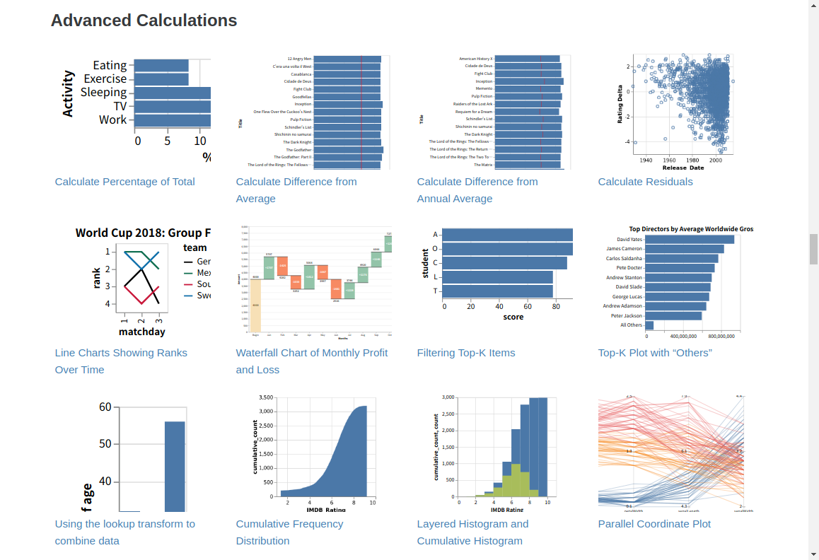
https://vega.github.io/vega-lite/examples/
(あった!)
「実験的な機能で、難しいんですけど、Vega Visualizationを使えばできるみたいですね(参考URLペタリ)」
『使い方教えてもらえます?』
「・・・」
というわけで、Kibana Vega Visualizationでウォーターフォールチャートを表示するのにチャレンジしてみます。
前提条件
- Elasticsearch 7.5.0
- Kibana 7.5.0
まずはVega-Lite公式サイトのExampleをKibanaで表示する
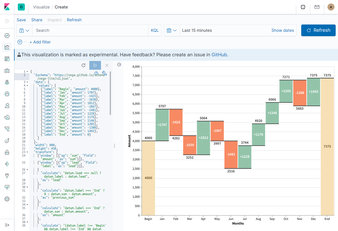
今回参考にするExampleはこれです。
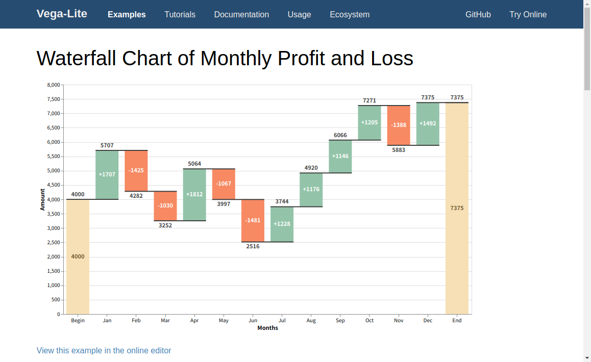
普段のKibanaの可視化よりもリッチな感じですね。
まずは、Kibanaで、このテストデータを可視化するところまで、進めてみたいと思います。
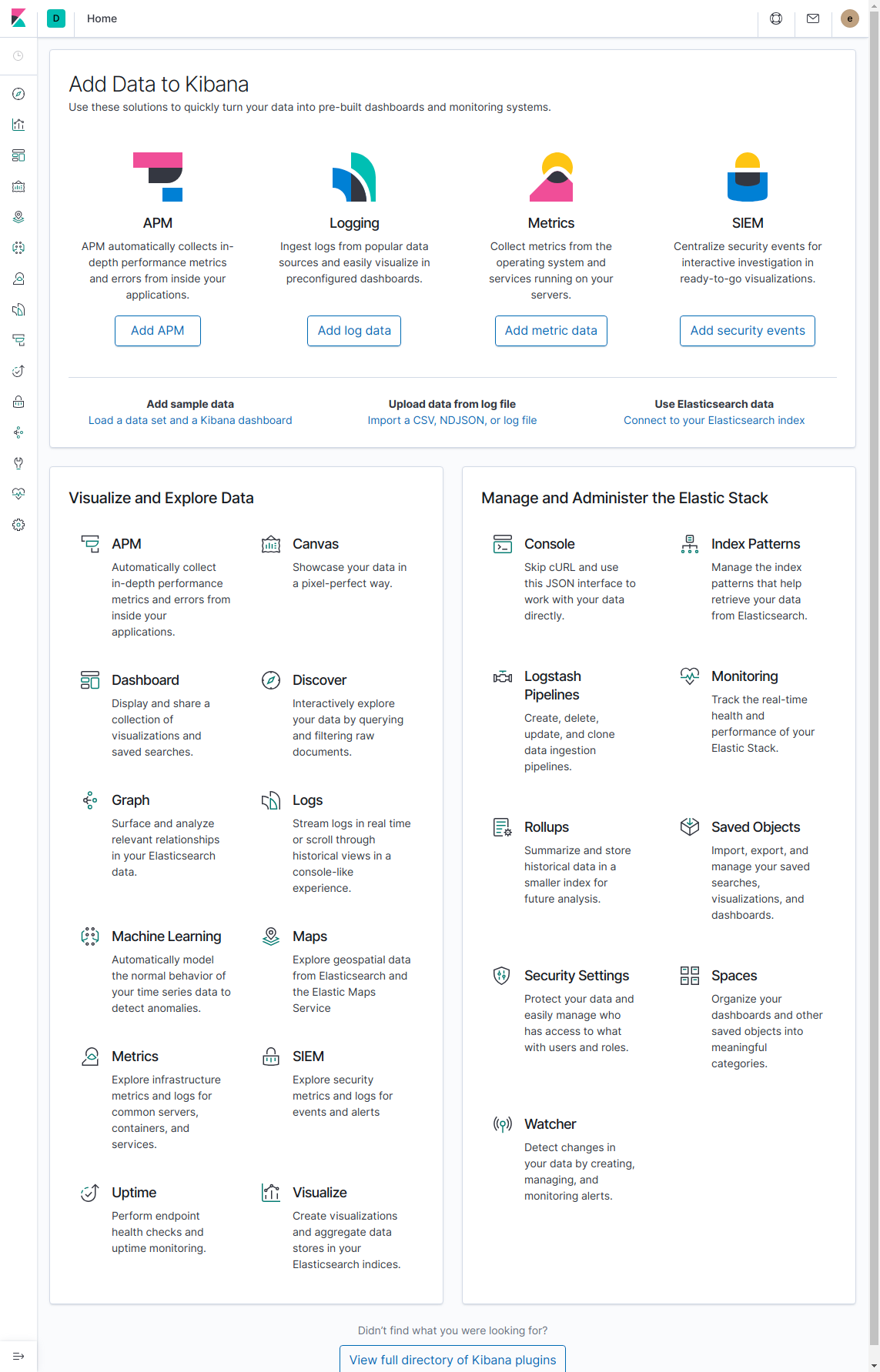
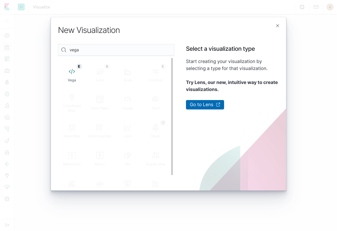
1. Kibanaにアクセスしてログインし、メニューからVisualizeをクリックする
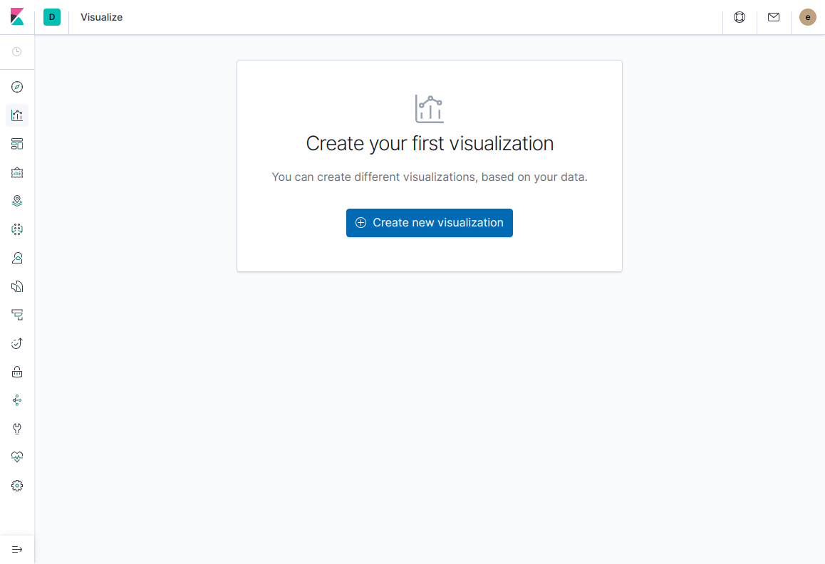
2. Create new visualizationをクリックする
3. Vegaをクリックする
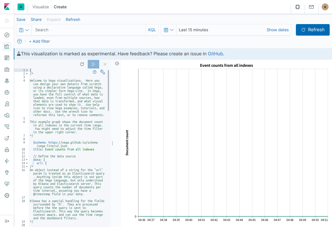
4. 画面左のコード部分にExampleページ下部に表示されているJSONをコピペする
5. Kibana 7.5.0に同梱されているVega-Liteのバージョンは2.6.0であるため、JSON内に記述されているschemaをv2に変更する
-   "$schema": "https://vega.github.io/schema/vega-lite/v4.json",
+   "$schema": "https://vega.github.io/schema/vega-lite/v2.json",
6. 再生ボタンをクリックして反映する
こんな感じで、Exampleをそのまま持ってくるだけなら簡単です。
これだけでも、こんな可視化もできるんですよ、というデモ用には使えるかもしれません。
テストデータをElasticsearchに投入し、それを可視化してみる
そのまま一足飛びに、Aggregationなどを駆使して可視化しても良いのですが、段階的に理解するために、テストデータをそのままElasticsearchに投入して、JSONの中ではなく、Elasticsearchの中から取得したドキュメントをVega Visualizationで可視化してみます。
1. bulk APIでElasticsearchにテストデータを投入する
KibanaのConsoleで以下を実行すれば、データを投入できます。
POST _bulk
{"index":{"_index":"waterfall","_id":"1"}}
{"label":"Begin","amount":4000}
{"index":{"_index":"waterfall","_id":"2"}}
{"label":"Jan","amount":1707}
{"index":{"_index":"waterfall","_id":"3"}}
{"label":"Feb","amount":-1425}
{"index":{"_index":"waterfall","_id":"4"}}
{"label":"Mar","amount":-1030}
{"index":{"_index":"waterfall","_id":"5"}}
{"label":"Apr","amount":1812}
{"index":{"_index":"waterfall","_id":"6"}}
{"label":"May","amount":-1067}
{"index":{"_index":"waterfall","_id":"7"}}
{"label":"Jun","amount":-1481}
{"index":{"_index":"waterfall","_id":"8"}}
{"label":"Jul","amount":1228}
{"index":{"_index":"waterfall","_id":"9"}}
{"label":"Aug","amount":1176}
{"index":{"_index":"waterfall","_id":"10"}}
{"label":"Sep","amount":1146}
{"index":{"_index":"waterfall","_id":"11"}}
{"label":"Oct","amount":1205}
{"index":{"_index":"waterfall","_id":"12"}}
{"label":"Nov","amount":-1388}
{"index":{"_index":"waterfall","_id":"13"}}
{"label":"Dec","amount":1492}
{"index":{"_index":"waterfall","_id":"14"}}
{"label":"End","amount":0}
{"index":{"_index":"waterfall","_id":"15"}}
2. Vegaの中でElasticsearchからテストデータを取得する
ExampleのJSONでは、dataフィールドの中にvaluesというフィールドが存在し、その中にテストデータの配列が記述されていました。Visualizeの中に直接データを埋め込みたい場合はこれでも良いですが、別の場所からデータを取得するには異なる記述方法を用います。
どんな記述方法かというと、values内にて、urlフィールドでURLを指定すると、そのURLから取得したJSONレスポンスを可視化に利用できます。Elasticsearchにクエリを実行した結果をVega Visualizationで使いたい場合はこのurlフィールドに検索クエリの内容を定義すれば良いわけです。古事記にもそう書かれている。
dataフィールド配下を以下のように書き換えます。
   "data": {
-    "values": [
-      {"label": "Begin", "amount": 4000},
-      {"label": "Jan", "amount": 1707},
-      {"label": "Feb", "amount": -1425},
-      {"label": "Mar", "amount": -1030},
-      {"label": "Apr", "amount": 1812},
-      {"label": "May", "amount": -1067},
-      {"label": "Jun", "amount": -1481},
-      {"label": "Jul", "amount": 1228},
-      {"label": "Aug", "amount": 1176},
-      {"label": "Sep", "amount": 1146},
-      {"label": "Oct", "amount": 1205},
-      {"label": "Nov", "amount": -1388},
-      {"label": "Dec", "amount": 1492},
-      {"label": "End", "amount": 0}
-    ]
+    url: {
+      index: waterfall
+      size: 100
+    }
   },
この時点で実行すると、グラフは表示されなくなってしまいますが、Elasticsearchからデータは取得されるようになっています。
Google Chromeで実行している場合はDeveloper Toolを起動し、Console画面で以下のコマンドを実行してみてください。
VEGA_DEBUG.vegalite_spec.data.values.hits.hits
これで、テストデータの配列が表示されていれば、取得成功です。
また、コード例の中で自然に使っていますが、Vega Visualizationのコード内では必ずしもJSON記法である必要はなく、HJSON記法を使用することもできます。こちらの方がコメントも書けてリッチですが、Vega関連のツールに貼り付けたり、Dev ToolsのConsoleでElasticsearchにクエリ発行するときなどにJSONに変換する必要が出てくるので、ケースバイケースで使い分けましょう。
一応、KibanaのVega Visualization編集画面でもJSON <-> HJSONの変換は可能なので、正直どっちでも良いと思います。
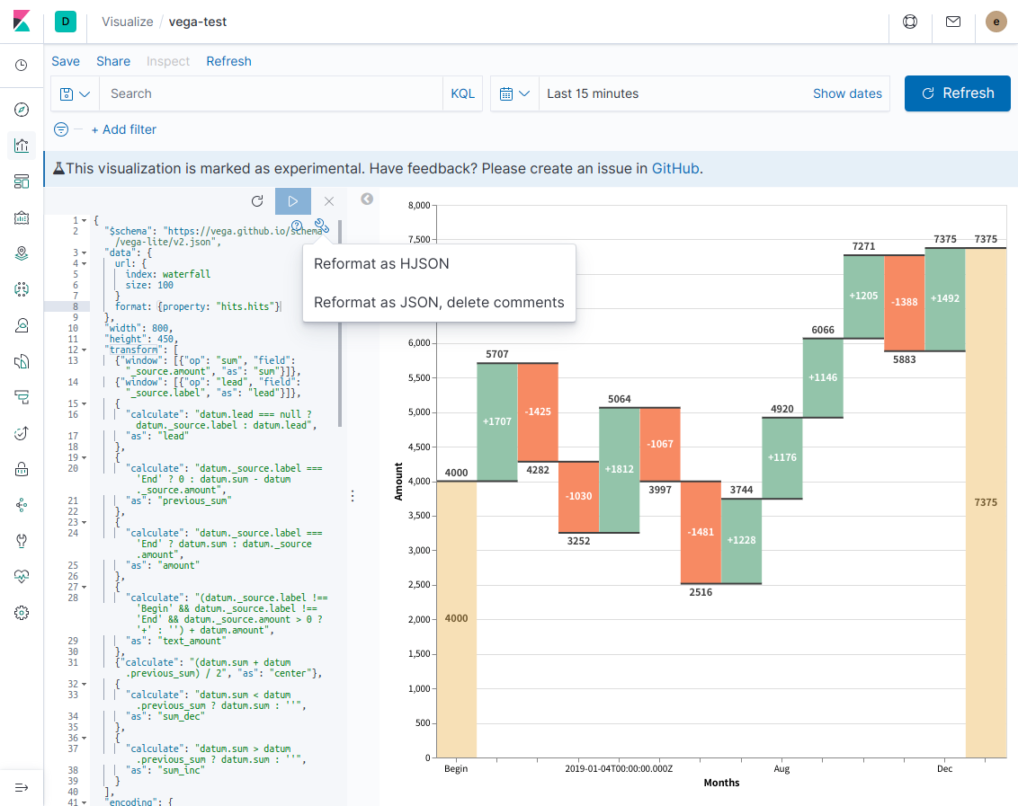
唯一、HJSON -> JSONの際にコメントが削除されることには注意が必要です。
3. 取得したテストデータを使ってグラフを表示する
では、いよいよ表示するデータを差し替えていきましょう。
まず、Elasticsearchの検索結果の中の何処にデータの配列が存在するかVegaに伝えてあげます。伝えるにはdataフィールドの中にformatというフィールドを定義し、そこにデータの配列までのパスを記述します。
 {
   "$schema": "https://vega.github.io/schema/vega-lite/v2.json",
   "data": {
     url: {
       index: waterfall
       size: 100
     }
+    format: {property: "hits.hits"}
   },
...skipping...
ご存知の方も多いと思いますが、Elasticsearchにクエリを実行すると、レスポンスの中のhits.hitsの中にデータの配列が存在します。
これを定義することでVegaがElasticsearchのデータを扱えるようになります。
次に元々JSON内部のデータを参照していた箇所をElasticsearchの取得結果を利用する形に変えてみます。元々は配列の直下にテストデータのフィールドが存在しましたが、Elasticsearchの検索結果では配列直下の_sourceの中にドキュメント自体のフィールドが存在します。したがって、以下のように書き換えれば良いです。
-
datum.label->datum._source.label -
"field": "label"->"field": "_source.label"
 {
   "$schema": "https://vega.github.io/schema/vega-lite/v2.json",
   "data": {
     url: {
       index: waterfall
       size: 100
     }
     format: {property: "hits.hits"}
   },
   "width": 800,
   "height": 450,
   "transform": [
-    {"window": [{"op": "sum", "field": "amount", "as": "sum"}]},
-    {"window": [{"op": "lead", "field": "label", "as": "lead"}]},
+    {"window": [{"op": "sum", "field": "_source.amount", "as": "sum"}]},
+    {"window": [{"op": "lead", "field": "_source.label", "as": "lead"}]},
     {
-      "calculate": "datum.lead === null ? datum.label : datum.lead",
+      "calculate": "datum.lead === null ? datum._source.label : datum.lead",
       "as": "lead"
     },
     {
-      "calculate": "datum.label === 'End' ? 0 : datum.sum - datum.amount",
+      "calculate": "datum._source.label === 'End' ? 0 : datum.sum - datum._source.amount",
       "as": "previous_sum"
     },
     {
-      "calculate": "datum.label === 'End' ? datum.sum : datum.amount",
+      "calculate": "datum._source.label === 'End' ? datum.sum : datum._source.amount",
       "as": "amount"
     },
     {
-      "calculate": "(datum.label !== 'Begin' && datum.label !== 'End' && datum.amount > 0 ? '+' : '') + datum.amount",
+      "calculate": "(datum._source.label !== 'Begin' && datum._source.label !== 'End' && datum._source.amount > 0 ? '+' : '') + datum.amount",
       "as": "text_amount"
     },
     {"calculate": "(datum.sum + datum.previous_sum) / 2", "as": "center"},
     {
...skipping...
         "strokeWidth": 2,
         "xOffset": -22.5,
         "x2Offset": 22.5
       },
       "encoding": {
         "x2": {"field": "lead"},
         "y": {"field": "sum", "type": "quantitative"}
       }
     },
     {
       "mark": {"type": "text", "dy": -4, "baseline": "bottom"},
       "encoding": {
         "y": {"field": "sum_inc", "type": "quantitative"},
         "text": {"field": "sum_inc", "type": "nominal"}
       }
     },
     {
       "mark": {"type": "text", "dy": 4, "baseline": "top"},
       "encoding": {
         "y": {"field": "sum_dec", "type": "quantitative"},
         "text": {"field": "sum_dec", "type": "nominal"}
       }
     },
     {
       "mark": {"type": "text", "fontWeight": "bold", "baseline": "middle"},
       "encoding": {
         "y": {"field": "center", "type": "quantitative"},
         "text": {"field": "text_amount", "type": "nominal"},
         "color": {
           "condition": [
             {
-              "test": "datum.label === 'Begin' || datum.label === 'End'",
+              "test": "datum._source.label === 'Begin' || datum._source.label === 'End'",
               "value": "#725a30"
             }
           ],
           "value": "white"
         }
       }
     }
   ],
   "config": {"text": {"fontWeight": "bold", "color": "#404040"}}
 }
変更した後、再生ボタンをクリックして反映します。
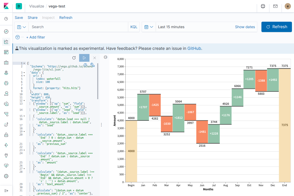
ここまでできると、外部スクリプトなりで今回投入したデータの形式でElasticsearchに投入することで、リアルタイムなデータ反映が可能になります。
しかしながら、せっかくKibanaで可視化するなら、ちゃんとtime filterに応じて表示期間が変わってほしいですし、外部スクリプトの力など借りなくともElasticsearchのAggregationで月ごとの集計はできるはずですよね?
やってみましょう。
日毎のデータを投入し、月別にAggregationした結果を可視化する
それでは、最後にKibanaのグラフらしい形に書き換えていきましょう。
- 月ごとの集計結果ではなく、日毎のデータが投入される前提とする
- 各月の集計はAggregationで行うようにする
- Kibana画面右上のtime filterが反映されるようにする
これらを達成できれば、十分KibanaのDashboard内で使える形になるでしょう。
1. Elasticsearchに日毎のデータを投入する
各月のAmountの合計値をグラフに表示しますが、ここに貼り付けられる範囲内のデータとするために各月2件のデータとします。Beginのデータに相当する部分は1年前の12月のデータであると仮定しました。
POST _bulk
{"index":{"_index":"time-series-waterfall","_id":"1"}}
{"timestamp": "2018-12-01","amount":2000}
{"index":{"_index":"time-series-waterfall","_id":"2"}}
{"timestamp": "2018-12-02","amount":2000}
{"index":{"_index":"time-series-waterfall","_id":"3"}}
{"timestamp": "2019-01-01","amount":3000}
{"index":{"_index":"time-series-waterfall","_id":"4"}}
{"timestamp": "2019-01-02","amount":2707}
{"index":{"_index":"time-series-waterfall","_id":"5"}}
{"timestamp": "2019-02-01","amount":2200}
{"index":{"_index":"time-series-waterfall","_id":"6"}}
{"timestamp": "2019-02-02","amount":2082}
{"index":{"_index":"time-series-waterfall","_id":"7"}}
{"timestamp": "2019-03-01","amount":2200}
{"index":{"_index":"time-series-waterfall","_id":"8"}}
{"timestamp": "2019-03-02","amount":1052}
{"index":{"_index":"time-series-waterfall","_id":"9"}}
{"timestamp": "2019-04-01","amount":2000}
{"index":{"_index":"time-series-waterfall","_id":"10"}}
{"timestamp": "2019-04-02","amount":3064}
{"index":{"_index":"time-series-waterfall","_id":"11"}}
{"timestamp": "2019-05-01","amount":2900}
{"index":{"_index":"time-series-waterfall","_id":"12"}}
{"timestamp": "2019-05-02","amount":1097}
{"index":{"_index":"time-series-waterfall","_id":"13"}}
{"timestamp": "2019-06-01","amount":1500}
{"index":{"_index":"time-series-waterfall","_id":"14"}}
{"timestamp": "2019-06-02","amount":1016}
{"index":{"_index":"time-series-waterfall","_id":"15"}}
{"timestamp": "2019-07-01","amount":2700}
{"index":{"_index":"time-series-waterfall","_id":"16"}}
{"timestamp": "2019-07-02","amount":1044}
{"index":{"_index":"time-series-waterfall","_id":"17"}}
{"timestamp": "2019-08-01","amount":2900}
{"index":{"_index":"time-series-waterfall","_id":"18"}}
{"timestamp": "2019-08-02","amount":2020}
{"index":{"_index":"time-series-waterfall","_id":"19"}}
{"timestamp": "2019-09-01","amount":3000}
{"index":{"_index":"time-series-waterfall","_id":"20"}}
{"timestamp": "2019-09-02","amount":3066}
{"index":{"_index":"time-series-waterfall","_id":"21"}}
{"timestamp": "2019-10-01","amount":3200}
{"index":{"_index":"time-series-waterfall","_id":"22"}}
{"timestamp": "2019-10-02","amount":4071}
{"index":{"_index":"time-series-waterfall","_id":"23"}}
{"timestamp": "2019-11-01","amount":3800}
{"index":{"_index":"time-series-waterfall","_id":"24"}}
{"timestamp": "2019-11-02","amount":2083}
{"index":{"_index":"time-series-waterfall","_id":"25"}}
{"timestamp": "2019-12-01","amount":3300}
{"index":{"_index":"time-series-waterfall","_id":"26"}}
{"timestamp": "2019-12-02","amount":4075}
2. Aggregationした結果を取得するようにする
時系列的に前との差分値を算出するにはElasticsearchのSerial differencing aggregationを使えば実現できそうです。
その他、色々と考慮事項はありましたが、試行錯誤して出来上がったHJSONがこちらです。
ポイントがある場所はコメントを記載しています。
{
  $schema: https://vega.github.io/schema/vega-lite/v2.json
  data: {
    url: {
      # この2つの設定を記述することでVega VisualizationにもKibanaのtime filterを反映することができる。
      %context%: true
      %timefield%: timestamp

      # 各月ごとにamountの加算値と前月との差分値を算出する。
      index: time-series-waterfall
      body: {
        # Aggregation以外の検索結果は不要なので、`size`は0にする。
        size: 0
        aggs: {
          month_date_histogram_of_timestamp: {
            # ドキュメントを月ごとにまとめる。
            date_histogram: {field: "timestamp", calendar_interval: "month"}
            aggs: {
              # 月ごとに分割されたドキュメントをそれぞれ加算する。
              sum_of_amount: {
                sum: {field: "amount"}
              }
              # 月ごとに加算された結果について、前の月との差分値を算出する。
              serial_diff_of_sum_of_amount: {
                serial_diff: {buckets_path: "sum_of_amount", lag: 1}
              }
            }
          }
        }
      }
    }

    # Aggregationの結果の配列部分を指定する。
    format: {
      property: aggregations.month_date_histogram_of_timestamp.buckets
    }
  }
  width: 800
  height: 450
  transform: [
    # 最後の月のデータであることを確認するために、次のデータの月があるかどうかを取得しておく。
    # `lead`オペレーションは次のデータの特定フィールドの値を取得できる命令で、次のデータがない場合には`null`が入る。
    # 当初はこの値を使うことで、最後のデータのみ複製して一番右に表示したかったが、現在は挫折中。
    # ただし、`window`で取得した値でなければ棒グラフ上下の黒線を意図した位置に配置できなかったため、可視化のためにこのフィールドを残すことにする。
    # 最後の列に`null`が表示されて死ぬほどダサいが我慢する。
    {
      window: [
        {
          op: lead
          field: key_as_string
          offset: 1
          as: next_lead
        }
      ]
    }

    # `sum`は既にElasticsearch側で計算済みであるため、そちらを使う。
    {
      calculate: "datum.sum_of_amount.value",
      as: "sum"
    }

    # X軸のラベルとしては日付文字列(`lead`)を使用する。
    {
      calculate: "datum.key_as_string",
      as: "lead"
    }

    # 以後、複数の場所で同様だが、最初の結果であるかどうかは`serial_diff_of_sum_of_amount`の結果が存在するかどうか、で判定する。
    # Serial Differencing Aggregationは配列の1件目には結果を返却しないため、そのチェックをすれば良い。
    {
      calculate: datum.serial_diff_of_sum_of_amount != null ? datum.sum - datum.serial_diff_of_sum_of_amount.value : 0
      as: previous_sum
    }
    {
      calculate: datum.serial_diff_of_sum_of_amount != null ? datum.serial_diff_of_sum_of_amount.value :datum.sum
      as: amount
    }
    {
      calculate: (datum.serial_diff_of_sum_of_amount != null && datum.amount > 0 ? '+' : '') + datum.amount
      as: text_amount
    }
    {
      calculate: (datum.sum + datum.previous_sum) / 2
      as: center
    }
    {
      calculate: datum.sum < datum.previous_sum ? datum.sum : ''
      as: sum_dec
    }
    {
      calculate: datum.sum > datum.previous_sum ? datum.sum : ''
      as: sum_inc
    }
  ]
  encoding: {
    x: {
      field: key_as_string
      type: ordinal
      sort: null
      axis: {labelAngle: 0, title: "Months"}
    }
  }
  layer: [
    {
      mark: {type: "bar", size: 45}
      encoding: {
        y: {field: "previous_sum", type: "quantitative", title: "Amount"}
        y2: {field: "sum"}
        color: {
          condition: [
            {
              test: datum.serial_diff_of_sum_of_amount == null
              value: "#f7e0b6"
            }
            {test: "datum.sum < datum.previous_sum", value: "#f78a64"}
          ]
          value: "#93c4aa"
        }
      }
    }
    {
      mark: {
        type: rule
        opacity: 1
        color: "#404040"
        strokeWidth: 2
        xOffset: -22.5
        x2Offset: 22.5
      }
      encoding: {
        # `x2`にElasticsearchから取得したラベル名をそのまま使ったところ、
        # 要素の配置が列名の左端から開始されてしまい、`Offset`の値を調整しても歪なグラフになってしまった。
        # Exampleと同様に、`window`で取得した値だとExampleと同様に列名のちょうど中間の位置に配置することができるようなので、
        # `lead`ではなく、`next_lead`を使用する。
        x2: {field: "next_lead"}
        y: {field: "sum", type: "quantitative"}
      }
    }
    {
      mark: {type: "text", dy: -4, baseline: "bottom"}
      encoding: {
        y: {field: "sum_inc", type: "quantitative"}
        text: {field: "sum_inc", type: "nominal"}
      }
    }
    {
      mark: {type: "text", dy: 4, baseline: "top"}
      encoding: {
        y: {field: "sum_dec", type: "quantitative"}
        text: {field: "sum_dec", type: "nominal"}
      }
    }
    {
      mark: {type: "text", fontWeight: "bold", baseline: "middle"}
      encoding: {
        y: {field: "center", type: "quantitative"}
        text: {field: "text_amount", type: "nominal"}
        color: {
          condition: [
            {
              test: datum.serial_diff_of_sum_of_amount == null
              value: "#725a30"
            }
          ]
          value: white
        }
      }
    }
  ]
  config: {
    text: {fontWeight: "bold", color: "#404040"}
  }
}
この内容をコピペして再生ボタンをクリックし、反映します。
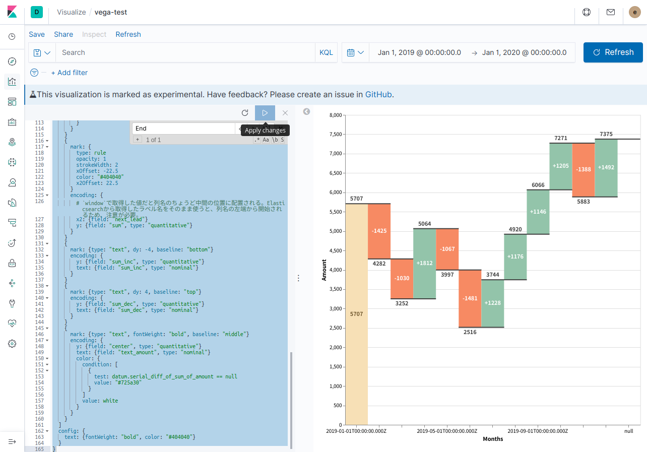
…あれ?元々のイメージと結果違ってない???
はい。右端の合計値を表示することはできなかったよ…頑張ってみましたが、僕の限界はここまでのようです…nullとか出ちゃってるしね _(:3」∠)_
ですが、一応Elasticsearchに入った日毎のデータをAggregationして、Vega Visualizationで可視化することはできました。右端部分以外はExampleと全く同じ表示のはずです。
では、最後に右上のtime filterを変更して、ちゃんと期間が反映されるか確認してみます。
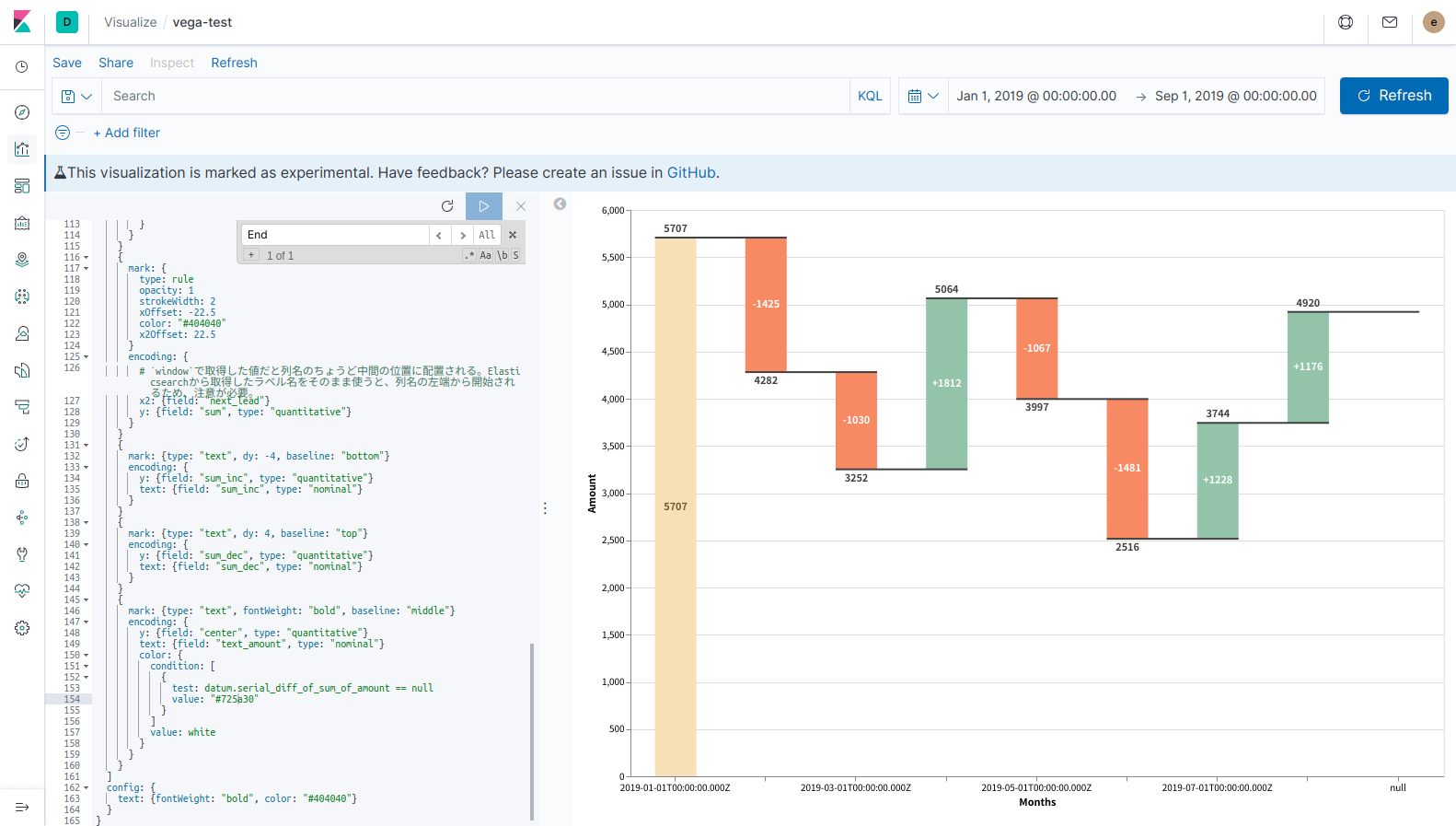
ちゃんと反映できてますね。良かった!
おわりに
Vega Visualization、まともに入門していなかったのですが、これでExampleを転用するぐらいのことはできるようになりました。非常に強力な機能なので、ぜひ皆さんも使ってみてはいかがでしょうか。
…果たしてExperimentalの印が外れる日は来るのか…。
最後に細かい話を1つ。Kibanaのtime filterに応じて表示期間を変更できるようになると、よりKibanaのDashboardに配置した際の利便性が向上するわけですが、必ずしも良いことだけではないようです。今回使用したままのグラフで、表示する月数を増やしたり狭めたりすると、このようになります。
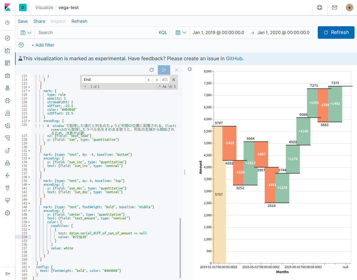
配置されている矩形の横幅と、上下の黒線がはみ出してしまっていますね。矩形を配置する場合、横幅をsizeというパラメータで指定するのですが、それをデータ件数に応じて変更する必要があるかもしれません。また、黒線の配置では長さの調整のために、オフセットを指定しているのですが、固定値であるため、現状は幅の変更に耐えられない作りになっています。
更に、それらを解決できたとしても、毎回必ず綺麗に表示できるかというと様々なコーナーケースが発生しそうです。あまり考えたくありません。
したがって、Vega Visualizationを使おうとする場合には
- まず、Vega Visualization以外のVisualizeで代替できないか、本当にそのグラフが必要なのか議論する
- できるだけ、Kibanaのtime filterを変更しても表示するグラフの形が変わらないようにする
- 横軸が時間のグラフを表示する場合には、データ数によってサイズを調整する必要がある棒グラフではなく、折れ線グラフなど、よりシンプルなグラフで表示する
- 横軸が時間のグラフで、どうしてもサイズの調整が必要な図形を配置したい場合は、毎回固定期間のtime filter(必ず1年で表示するなど)で利用する
ことを検討したほうが良いのではないか、と感じました。これらがどれもNGだった場合は、幅職人になる覚悟を決めましょう。(もしかしたらautosizeとか使ったら簡単に実現できるんだろうか)
ところで、今回はVega-LiteのExampleを転用する話でしたが、VegaのExampleだとどんなところが違ったりするんでしょうか。また、試してみたいと思います。
Advent Calendar、明日は@shin0higuchiさんの記事です。お楽しみに!
Appendix
Translateしたデータの変換後の結果が確認したい
ブラウザの開発者ツールからhttps://t.co/WxLwcuGlaBかなにかで見られた気がしますhttps://t.co/jKcU3QPAn1
— shin higuchi @Acroquest (@shin0higuchi) December 14, 2019
明日のAdvent Calendar投稿者でもある、@shin0higuchiさんから情報提供いただきました。ありがとうございます!
大体の確認したいデータはVEGA_DEBUG.view._runtimeで見ることができるみたいです。データのみに着目して確認したい場合はVEGA_DEBUG.view._runtime.data。その他、よく確認したいデバッグ値については「Vega利用時によくある7つの疑問 - Taste of Tech Topics」を確認しておくと幸せになれます。