はじめに
今までQGISを使って地理空間情報データの処理をしていましたが、Rに地理空間情報のデータ処理を行うことができるパッケージが存在すると聞きました。
色々と記事になっているとは思いますが、自身の備忘録として、書き留めたいと思います。
※DataCampの
Spatial Analysis with sf and raster in Rの一連の流れを自分用にメモしたものです。したがって、取扱うデータはオープンデータ等ではなく、DataCampが用意シているデータをそのまま使います。
ベクターデータの読み取り
Rのsfパッケージを使うことで、Rで地理空間情報を読み込むことができます。
使用する関数名:st_read()
st_read()を使用することで、地理空間情報(シェープファイル)を読み込むことが可能です。シェープファイルは、ポイントを示すデータ、ラインを示すデータ、ポリゴンを示すデータの3つがありますが、全て読み込むことが可能です。
ファイルを読み込むと、ファイルに関するメタデータが表示されます。
また、Rのデータフレームが表示され、ジオメトリ列が表示されます。
# Load the sf package
library(sf)

# Read in the trees shapefile
trees <- st_read("trees.shp")

# Read in the neighborhood shapefile
neighborhoods <- st_read("neighborhoods.shp")

# Read in the parks shapefile
parks <- st_read("parks.shp")

# View the first few trees
head(trees)
結果は下記の通り
> head(trees)
Simple feature collection with 6 features and 7 fields
geometry type:  POINT
dimension:      XY
bbox:           xmin: -74.13116 ymin: 40.62351 xmax: -73.80057 ymax: 40.77393
epsg (SRID):    4326
proj4string:    +proj=longlat +ellps=WGS84 +no_defs
  tree_id  nta longitude latitude stump_diam      species      boroname
1  558423 QN76 -73.80057 40.67035          0  honeylocust        Queens
2  286191 MN32 -73.95422 40.77393          0 Callery pear     Manhattan
3  257044 QN70 -73.92309 40.76196          0  Chinese elm        Queens
4  603262 BK09 -73.99866 40.69312          0       cherry      Brooklyn
5   41769 SI22 -74.11773 40.63166          0       cherry Staten Island
6   24024 SI07 -74.13116 40.62351          0    red maple Staten Island
                    geometry
1 POINT (-73.80057 40.67035)
2 POINT (-73.95422 40.77393)
3 POINT (-73.92309 40.76196)
4 POINT (-73.99866 40.69312)
5 POINT (-74.11773 40.63166)
6 POINT (-74.13116 40.62351)
結果として出力されるのは、ジオメトリタイプやバウンティボックスの座標、EPSG番号や投影・座標系情報が出力されるみたいですね。
また、それ以外にもtree_id毎の各種データが出力されることがわかりました。ogr2ogrでもわかることですが、Rでのプログラムを慣れている人であれば、こちらを使うのもよいなと思いました。
ラスターデータの読み取り
「ラスター」とは衛星画像・航空写真などを示すデータです。Rではラスターパッケージを使うことでラスターデータを処理することができます。
ラスターデータを使用する場合、覚えておくべき最も重要なことの1つは、「シングルバンド」「マルチバンド」という2つのデータがあります。
「シングルバンド」は、例えば白と黒の2つからなるグレースケール画像。
「マルチバンド」は、例えば赤(R)、緑(G)、青(B)からなるカラースケール画像です。
ラスターデータにおけるシングルバンドデータの典型的な例は、各ピクセル値がその位置の標高を示す標高ラスターです。(例えばSRTMのようなデータ)
マルチバンドラスターには、R,G,B以外に、複数のレイヤーを持つことが多いです。
使用する関数名:raster(),blick()
# Load the raster package
library(raster)

# Read in the tree canopy single-band raster
canopy <- raster("canopy.tif")

# Read in the manhattan Landsat image multi-band raster
manhattan <- brick("manhattan.tif")

# Get the class for the new objects
class(canopy)
class(manhattan)

# Identify how many layers each object has
nlayers(canopy)
nlayers(manhattan)
※個人的気になったメモ;
■ライブラリ名がrasterでシングルバンドデータを読み込むときの関数名がrasterと同じ名前のものを使う。困惑しそう。
結果は以下の通り
# Load the raster package
library(raster)

# Read in the tree canopy single-band raster
canopy <- raster("canopy.tif")

# Read in the manhattan Landsat image multi-band raster
manhattan <- brick("manhattan.tif")

# Get the class for the new objects
class(canopy)
class(manhattan)

# Identify how many layers each object has
nlayers(canopy)
nlayers(manhattan)
sfオブジェクトの取扱い
sfオブジェクトは、地理空間特有のプロパティは持つものの、単なるデータフレームです。これは、dplyrパッケージを使用してsfオブジェクトを操作できるということです。
そのため、dplyr関数のselectを使用して変数を選択またはドロップし、 filterを使用してデータフィルタリングをし、mutateを使用して列を追加変更することが可能です。
さらに、パイプ演算子(%>%) を使用してコードを簡素化することもできます。
使用する関数名:select,filter
# Load the sf package
library(sf)

# ... and the dplyr package
library(dplyr)

# Read in the trees shapefile
trees <- st_read("trees.shp")

# Use filter() to limit to honey locust trees
honeylocust <- trees %>% filter(species == "honeylocust")

# Count the number of rows
nrow(honeylocust)

# Limit to tree_id and boroname variables
honeylocust_lim <- honeylocust %>% select(tree_id, boroname)

# Use head() to look at the first few records
head(honeylocust_lim)
結果は下記の通り
> head(honeylocust_lim)
Simple feature collection with 6 features and 2 fields
geometry type:  POINT
dimension:      XY
bbox:           xmin: -73.97524 ymin: 40.67035 xmax: -73.80057 ymax: 40.83136
epsg (SRID):    4326
proj4string:    +proj=longlat +ellps=WGS84 +no_defs
  tree_id boroname                   geometry
1  558423   Queens POINT (-73.80057 40.67035)
2  548625 Brooklyn POINT (-73.97524 40.68575)
3  549439 Brooklyn POINT (-73.94137 40.67557)
4  181757 Brooklyn POINT (-73.89377 40.67169)
5  379387   Queens  POINT (-73.8221 40.69365)
6  383562    Bronx POINT (-73.90041 40.83136)
>
sfオブジェクトのジオメトリ列について
sfの良きところは、空間オブジェクトがデータフレームであるところです。ジオメトリはリスト列に保存されています。
リスト列は、1つの変数に多くの情報を保存することができます。
※dplyr::tbl_df()は非推奨のため、tibble::as_tibble()を使用しtibbleに変換します。
使用する関数名:tibble(),as_tibble()
# Create a standard, non-spatial data frame with one column
df <- tibble(a = 1:3)

# Add a list column to your data frame
df$b <- list(1:4, 1:5, 1:10)

# Look at your data frame with head
head(df)

# Convert your data frame to a tibble and print on console
as_tibble(df)

# Pull out the third observation from both columns individually
df$a[3]
df$b[3]
結果は下記の通り
> # Create a standard, non-spatial data frame with one column
> df <- tibble(a = 1:3)
>
> # Add a list column to your data frame
> df$b <- list(1:4, 1:5, 1:10)
>
> # Look at your data frame with head
> head(df)
# A tibble: 3 x 2
      a b
  <int> <list>
1     1 <int [4]>
2     2 <int [5]>
3     3 <int [10]>
>
> # Convert your data frame to a tibble and print on console
> as_tibble(df)
# A tibble: 3 x 2
      a b
  <int> <list>
1     1 <int [4]>
2     2 <int [5]>
3     3 <int [10]>
>
> # Pull out the third observation from both columns individually
> df$a[3]
[1] 3
> df$b[3]
[[1]]
 [1]  1  2  3  4  5  6  7  8  9 10
>
※データフレームの1要素をリストとし、そこにジオメトリ情報(緯度経度等)を入れるようにしている。
ベクターレイヤーから幾何情報を抽出する
sfには、ベクターから面積などの幾何学的情報にアクセスできる関数があります。
例えば、関数st_areaおよび関数st_lengthはそれぞれベクターフィーチャの面積と長さを返します。
st_area()やst_length()などの関数の結果はベクトルではないことにc獣医する必要があります。代わりに、結果にはユニットのクラスがあります。つまり、ベクトルの結果には、オブジェクトのユニットを記述するメタデータが付随します。
メタデータが付随するため、以下のようなコードは動きまません
例1
# This will not work
result <- st_area(parks)
result > 30000
代わりに、関数unclass()を使用し、ユニットを削除する必要があります。
例2
# This will work
val <- 30000
unclass(result) > val
または、valのクラスを単位に変換する必要があります。次に例を示します。
例3
# This will work
units(val) <- units(result)
result > val
使用する関数名:st_area(),unclass(),st_geometry()
# Read in the parks shapefile
parks <- st_read("parks.shp")

# Compute the areas of the parks
areas <- st_area(parks)

# Create a quick histogram of the areas using hist
hist(areas, xlim = c(0, 200000), breaks = 1000)

# Filter to parks greater than 30000 (square meters)
big_parks <- parks %>% filter(unclass(areas) > 30000)

# Plot just the geometry of big_parks
plot(st_geometry(big_parks))
結果は、下記の画像が出力される


※ここまで来ると、実際のデータ分析に使えそうだなと感じました。QGIS上でも、ベクターレイヤーから条件を設定して表示/非表示にすることを自身では頻繁にやっています。Rでもこのような処理ができたら楽だと思っていましたが、
st_areaで面積を求め、
filterで面積を絞り、
st_geometryとplotを使うことで
実現可能だということが理解できました。
そういえばQGISでもフィールド計算機?で$areaと打てば面積が出せるとか、ありましたよね。それと同じですね。
ベクトル空間オブジェクトを可視化
Rを使ってクイックマップやプロットを作成するための関数はplot()です。例えば、plot(my_data)と実行すれば空間オブジェクトを表示することができます。しかし、デフォルト設定では想定していたプロットはできない場合があります。plot()関数をsfオブジェクトに適用すると、データの各属性に1つずつマップのセットが作成されます。代わりに、単一の属性のマップを作成する場合、例としてplot(my_data["my_variable"])を使用することで、その属性を抽出可能です。
多くの場合、属性の色分けなしで未加工のジオメトリをプロットするだけです。未加工のジオメトリをプロットするだけです。(例えば、ポイント属性のジオメトリマップに、市区町村の境界を追加するなど)このため、st_geometry()関数を使用して
ジオメトリを抽出し、結果をプロットできます。新しいオブジェクトを作成するか、plot()関数内でst_geometry()をネストします。
使用する関数名:plot(),st_geometry()
# Plot the parks object using all defaults
plot(parks)

# Plot just the acres attribute of the parks data
plot(parks["acres"])

# Create a new object of just the parks geometry
parks_geo <- st_geometry(parks)

# Plot the geometry of the parks data
plot(parks_geo)
結果は下記です。
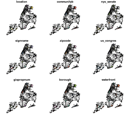
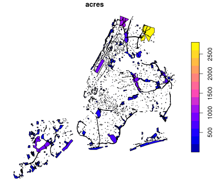

※読み込んだshpファイルをそのままplot()してしまうと、全要素に対するマップが作成されてしまいます。一つのattributeだけについてマップ作成する場合はplot(parks["acres"])のように、する必要があります。 (これって、plot(parks$acres)でも動作するんですかね?という疑問がありますが。。
白地図(何も要素を入れていないマップ)を表示させるためには、plot(st_geometry(parks))のようにst_geometry()を使えばよいということがわかりました。
ラスターデータについて学ぶ
ベクターデータはデータフレームとして扱うことができました。そのためdplyrをそのまま適用することができました。ラスターデータは、データとメタデータが格納できる特別に設計されたデータフレーム的なものを使います。
もちろんデータとメタデータはアクセス可能です。例えば、オブジェクトの空間範囲(バウンティボックスのような境界ボックス)はextent()でアクセスできます。crs()で座標参照系にアクセスできます。グリッドセルの数はncell()でアクセスできます。
使用する関数名:raster(),brick(),extent(),crs(),ncell()
# Load the raster package
library(raster)

# Read in the rasters
canopy <- raster("canopy.tif")
manhattan <- brick()("manhattan.tif")

# Get the extent of the canopy object
extent(canopy)

# Get the CRS of the manhattan object
crs(manhattan)

# Determine the number of grid cells in both raster objects
ncell(manhattan)
ncell(canopy)
結果は下記の通り
> # Load the raster package
> library(raster)
>
> # Read in the rasters
> canopy <- raster("canopy.tif")
> manhattan <- brick("manhattan.tif")
>
> # Get the extent of the canopy object
> extent(canopy)
class      : Extent
xmin       : 1793685
xmax       : 1869585
ymin       : 2141805
ymax       : 2210805
>
> # Get the CRS of the manhattan object
> crs(manhattan)
CRS arguments:
 +proj=utm +zone=18 +datum=WGS84 +units=m +no_defs +ellps=WGS84
+towgs84=0,0,0
>
> # Determine the number of grid cells in both raster objects
> ncell(manhattan)
[1] 619173
> ncell(canopy)
[1] 58190
>
ラスターデータ値へのアクセス
範囲と解像度(グリッドサイズ)によっては、ラスタデータが非常に大きくなります。これに対処するため、raster()およびbrick()関数は、必要に応じて実際のラスター値のみを読み込むように設計されています。 これが正しいことを示すために、オブジェクトでinMemory()関数が使用できます。値がメモリにない場合はFALSEを返します。
head()関数を使用する場合、ラスターパッケージは値の完全なセットではなく、必要な値のみを読み込みます。
ラスタ値は、それを必要とする空間解析操作を実行するか、関数getValues()を使用してラスタから値を手動で読み込むことができる場合、デフォルトで読み込まれます。
使用する関数名:inMemory(),head(),getValues(),hist()
# Check if the data is in memory
inMemory(canopy)

# Use head() to peak at the first few records
head(canopy)

# Use getValues() to read the values into a vector
vals <- getValues(canopy)

# Use hist() to create a histogram of the values
hist(vals)
結果は下記の通り。
# Check if the data is in memory
inMemory(canopy)

# Use head() to peak at the first few records
head(canopy)

# Use getValues() to read the values into a vector
vals <- getValues(canopy)

# Use hist() to create a histogram of the values
hist(vals)

※inMemory()の結果がFALSEだったため、全てのデータを読み込んでいるわkではないということがわかる。つまり、ラスターパッケージはメモリスペースを節約するために、必要に応じてラスター値のみを読み込んでいることがわかりました。getValues()を使うことで、値を手動で取得することができます。
ラスターオブジェクトをプロットする
ベクトルデータをマップ生成するのと同様に、ラスターデータもplot()関数を使用してマップ表示することができます。
ラスタパッケージには、シングルバンドとマルチバンドの両方のラスタをプロットするための便利なメソッドがあります。 シングルバンドラスターの場合、またはマルチバンドラスターの各レイヤーのマップの場合、単純にplot()を使用できます。 赤、緑、青のレイヤーを持つマルチバンドラスターがある場合、plotRGB()関数を使用して、ラスターレイヤーを1つの画像として一緒にプロットできます。
使用する関数名:plot(),plotRGB()
# Plot the canopy raster (single raster)
plot(canopy)

# Plot the manhattan raster (as a single image for each layer)
plot(manhattan)

# Plot the manhattan raster as an image
plotRGB(manhattan)
結果は下記の通り
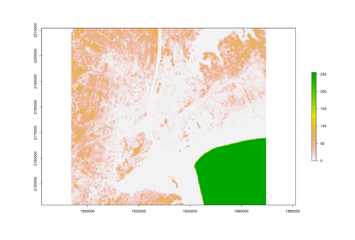
緑色になっている箇所はなんでしょうか。
ハズレ値的なものでしょうか。
本データを使ってヒストグラム等の処理をするときは、当該箇所を削除するなどの前処理加工をしてからの方が良さそうですね。
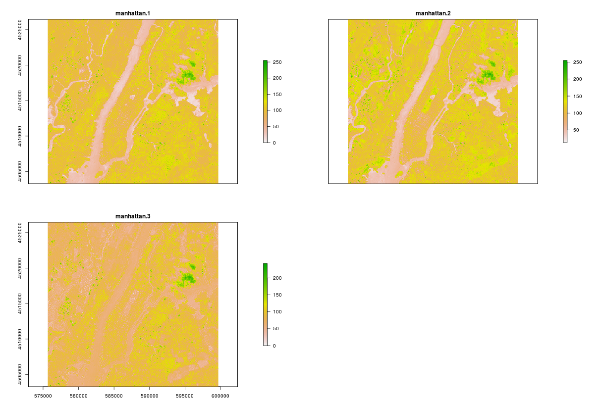
各レイヤーの単一レイヤーをプロットしていることがわかります。デフォルトのカラーバーがちょっとわかりにくいですが。。。
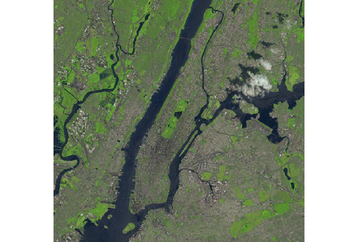
plotRGB()と関数が用意してあるのは便利でいいですね。
さくっとデータの確認ができそうです。
おわりに
Rを使った地理空間情報データの処理の基本的な部分はわかりました。データ読み込みや簡単なデータクレンジング、またラスターデータの表示等など、基本的な部分はわかったと思います。引き続き、備忘録を残していこうと思います。