前回のterraパッケージによる複数ラスタの一括読み込みの続きです。前回は複数の領域から複数のラスタを読み込む手法を紹介しました。今回は、このようにして読み込んだリスト形式のラスタスタックの値をベクトルポイントに付値する方法です。
全コード
# パッケージ読み込み
library(tidyverse)
library(terra)
library(sf)

# 遺跡データ読込
site <-
  st_read("site_point.gpkg") %>%
  dplyr::select(geom) %>% # 位置情報だけのデータに変換
  as("SpatVector")  # SpatVector形式に変換

# 遺跡ポイントをラスタでクリップ_結果のベクターは領域ごとのリスト形式
site_crop <-
  map(raster_list_stack,  # ラスタのリストをmap()の引数に指定
      terra::crop,  # 関数を記述
      x = site)   # terra::crop()の引数を指定

# terra::extract で遺跡ポイントにラスタを付値
site_crop_ext <- list() # 空のリストオブジェクト作成

# リストに格納されているベクタポイントにラスタを付値
for(i in 1:length(site_crop)){
  terra::extract(
    x = raster_list_stack[[i]],  # ラスタを格納したリスト
    y = site_crop[[i]]  # ベクタポイントを格納したリスト
  ) -> site_crop_ext[[i]]  # それぞれの結果はデータフレームに格納されるので、データフレムをさらにリストに格納
}

# 遺跡ポイントのデータフレームをunestしてtibble化
# 列名を同じにする
colName <-
  c("ID","aspect","DEM","irradiation","sky_view_factor",
    "slope","TRI" ,"wetness_index")
# for文でcolNameを代入
for(i in 1:length(site_crop_ext)){
  names(site_crop_ext[[i]]) <- colName
}

# 遺跡ポイントのリストを結合してtibble化
site_presence <-
  site_crop_ext %>%
  map_dfr(bind_rows) %>%
  mutate(presence = 1) %>%
  as_tibble() %>%
  dplyr::select(-ID)

# 不在データの作成
# bgはリスト形式でラスタごとにサンプリング
bg <-
  map(
    raster_list_stack,
    terra::spatSample,
    size = 100,
    na.rm = TRUE
      )

# for文でcolNameを代入_colNameは使いまわし
colName2 <-
  c("aspect","DEM","irradiation","sky_view_factor",
    "slope","TRI" ,"wetness_index")
for(i in 1:length(bg)){
  names(bg[[i]]) <- colName2
}
# 不在ポイントのリストを結合してtibble化してから遺跡ポイントと結合
data <-
  bg %>%
  map_dfr(bind_rows) %>%
  mutate(presence = 0) %>%  # presence = 0は遺跡なしをあらわす新しい変数
  as_tibble() %>%
  bind_rows(site_presence) %>%
  mutate(aspect = case_when(
    aspect == 1 ~ "East",
    aspect == 2 ~ "North",
    aspect == 3 ~ "West",
    aspect == 4 ~ "South"
  )) %>%
  mutate(presence_fact = case_when(
    presence == 1 ~ "presence",
    presence == 0 ~ "absence",
  ))
# 方位をrelevel
data$aspect <- fct_relevel(data$aspect,
                           "North", "East", "South", "West")
パッケージとデータ読み込み
tidyverseとterraを使います。sfはベクタデータの読み込みに使います。
library(tidyverse)
library(terra)
library(sf)
データは埋蔵文化財包蔵地(GISデータ)【北海道】をダウンロードして使用します。
site <-
  st_read("site_point.gpkg") %>%
  dplyr::select(geom) %>% # 位置情報だけのデータに変換
  as("SpatVector")  # SpatVector形式に変換
ラスタデータの領域でベクタポイントをクリップ
前回作成したリスト形式のラスタスタックの領域を利用して、ラスタと同一領域にあるベクタポイントだけを選択します。
# 遺跡ポイントをラスタでクリップ_結果のベクターは領域ごとのリスト形式
site_crop <-
  map(raster_list_stack,  # ラスタのリストをmap()の引数に指定
      terra::crop,  # 関数を記述
      x = site)   # terra::crop()の引数を指定
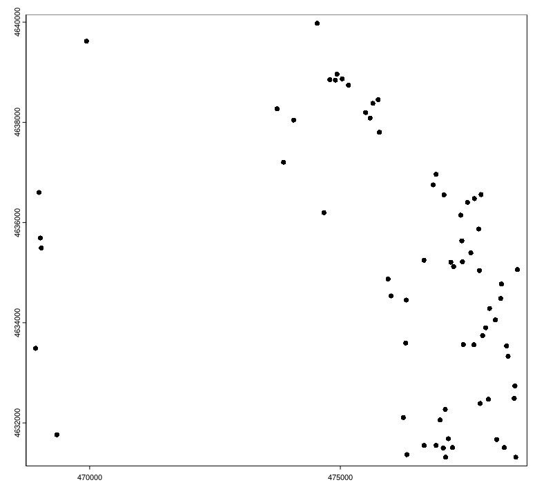
結果は領域ごとのリスト形式になっています。
plot(site_crop[[1]])
リストの1番目のポイント
遺跡ポイントにラスタ値を付値
リスト化された遺跡ポイントは、前回作成したラスタスタックと同じ領域です。遺跡ポイントと重なる位置にあるラスタ値を取得します。つまり、遺跡の標高や傾斜量、湿潤指標などのラスタ値を遺跡ポイントに結合することになります。
# terra::extract で遺跡ポイントにラスタを付値
site_crop_ext <- list() # 空のリストオブジェクト作成

# リストに格納されているベクタポイントにラスタを付値
for(i in 1:length(site_crop)){
  terra::extract(  # terra::extract関数でXのオブジェクトからYのオブジェクトに値を付値
    x = raster_list_stack[[i]],  # ラスタを格納したリスト
    y = site_crop[[i]]  # ベクタポイントを格納したリスト
  ) -> site_crop_ext[[i]]  # それぞれの結果はデータフレームに格納されるので、データフレームをさらにリストに格納
}
ここで使用しているterra::extract関数は、引数yに指定したオブジェクトに引数xに指定したオブジェクトの値を付値する関数です。
結果はデータフレームに格納されます。
> head(site_crop_ext[[1]])
  ID aspect      DEM irradiation sky_view_factor    slope       TRI wetness_index
1  1      3 99.01842    7614.385       0.9918564 2.231572 1.0466492     13.571608
2  2     NA 25.25573          NA       0.9994174       NA 0.1240834     14.125753
3  3      1 44.29057    7540.029       0.9950247 5.394267 2.5468919      7.523900
4  4      1 23.48900    7614.466       0.9995403 1.938430 0.8629836     10.541191
5  5      3 94.61606    7434.221       0.9763082 6.974305 3.0800574      8.252393
6  6      4 98.28577    7655.185       0.9913239 7.059281 3.1395702      7.748467
遺跡ポイントのデータフレームをunestしてtibble化する
ラスタの図角ごとにリスト化されているデータフレームを1つのテーブルに整形します。
列名を統一する
1つのテーブルに結合する前にcolnameを統一します。for文を回して処理しますが、もともと列名が統一されている場合はこの作業は不要です。
# 列名をcolNameオブジェクトに格納
colName <-
  c("ID","aspect","DEM","irradiation","sky_view_factor",
    "slope","TRI" ,"wetness_index")
# for文でcolNameを代入
for(i in 1:length(site_crop_ext)){
  names(site_crop_ext[[i]]) <- colName
}
遺跡ポイントのリストを結合してtibble化
site_presence <-
  site_crop_ext %>%
  map_dfr(bind_rows) %>%  # map_dfrは行結合
  mutate(presence = 1) %>%  # 遺跡在データなので新たなフィールドpresenceに1を代入する
  as_tibble() %>%
  dplyr::select(-ID)
site_presenceの中身は遺跡の地点における地形指標のデータフレームになっている。
> site_presence
# A tibble: 652 × 8
   aspect   DEM irradiation sky_view_factor slope   TRI wetness_index presence
    <dbl> <dbl>       <dbl>           <dbl> <dbl> <dbl>         <dbl>    <dbl>
 1      3  99.0       7614.           0.992  2.23 1.05          13.6         1
 2     NA  25.3         NA            0.999 NA    0.124         14.1         1
 3      1  44.3       7540.           0.995  5.39 2.55           7.52        1
 4      1  23.5       7614.           1.00   1.94 0.863         10.5         1
 5      3  94.6       7434.           0.976  6.97 3.08           8.25        1
 6      4  98.3       7655.           0.991  7.06 3.14           7.75        1
 7      3  96.7       7582.           0.981  3.97 1.75          10.6         1
 8      3  87.7       7613.           0.993  3.02 1.35          13.5         1
 9      3 105.        7622.           0.991  7.27 3.20          10.3         1
10      3 156.        7620.           0.991  7.96 3.52           7.73        1
# ℹ 642 more rows
# ℹ Use `print(n = ...)` to see more rows
不在データの作成
続いて、バックグラウンドとなる遺跡不在データ(正確には「偽不在」データ)を取得します。
ラスタからランダムに地形指標を取得
# bgはリスト形式でラスタごとにサンプリング
bg <-
  map(
    raster_list_stack,  # 第1引数はリスト化されたラスタスタック
    terra::spatSample,  # ランダムサンプリング
    size = 100,  # サンプリング数
    na.rm = TRUE
      )
bgはリスト形式でランダムサンプリングした地形指標が格納されます。
> bg
[[1]]
    aspect        DEM irradiation sky_view_factor        slope          TRI wetness_index
1        4 143.542923    7658.974       0.9939261 5.509160e+00 2.444514e+00      9.309402
2        2  33.199425    7602.284       0.9944703 8.439599e-01 3.904255e-01     11.985716
3        2  28.797836    7594.999       0.9969020 1.363700e+00 6.018501e-01     13.741795
4        4   7.866040    7603.917       0.9991269 2.759873e-01 1.341868e-01     16.425617
5        4 253.847275    7564.910       0.9689551 1.773701e+01 8.009809e+00      5.472491
6        3 115.580612    7625.082       0.9912611 1.031421e+01 4.577321e+00      6.057926
for文でcolNameを代入
遺跡データについて行ったのと同じ作業です。リスト内のcolnameを統一します。
colName2 <-
  c("aspect","DEM","irradiation","sky_view_factor",
    "slope","TRI" ,"wetness_index")
for(i in 1:length(bg)){
  names(bg[[i]]) <- colName2
}
遺跡不在データのリストを結合してtibble化してから遺跡在データと結合
少し長めの処理を回します。
- bgに格納された不在データのリストをデータフレーム化
- 遺跡不在を表す新たな変数作成
- 遺跡在データと結合
- 傾斜方位を名義変数化
- 在/不在を名義変数化
data <-
  bg %>%
  map_dfr(bind_rows) %>%  # リスト形式のデータをデータフレーム化
  mutate(presence = 0) %>%  # presence = 0は遺跡なしをあらわす新しい変数
  as_tibble() %>%  # tibble形式化
  bind_rows(site_presence) %>%  # 遺跡在データを結合
  mutate(aspect = case_when(  # 傾斜方位を名義変数化
    aspect == 1 ~ "East",
    aspect == 2 ~ "North",
    aspect == 3 ~ "West",
    aspect == 4 ~ "South"
  )) %>%
  mutate(presence_fact = case_when(  # 在/不在データを名義変数化
    presence == 1 ~ "presence",
    presence == 0 ~ "absence",
  ))
傾斜方位をrelevelする
傾斜方位を北から時計回りにrelevelします。fct_relevel関数はベクトルにしか適用できないのがちょっと残念です。
data$aspect <- fct_relevel(data$aspect,
                           "North", "East", "South", "West")
完成!!
遺跡在データと不在データが結合されたデータフレームが完成しました。次回はこのデータを可視化していきます。
> data
# A tibble: 1,552 × 9
   aspect    DEM irradiation sky_view_factor   slope    TRI wetness_index presence presence_fact
   <fct>   <dbl>       <dbl>           <dbl>   <dbl>  <dbl>         <dbl>    <dbl> <chr>
 1 South  144.         7659.           0.994  5.51   2.44            9.31        0 absence
 2 North   33.2        7602.           0.994  0.844  0.390          12.0         0 absence
 3 North   28.8        7595.           0.997  1.36   0.602          13.7         0 absence
 4 South    7.87       7604.           0.999  0.276  0.134          16.4         0 absence
 5 South  254.         7565.           0.969 17.7    8.01            5.47        0 absence
 6 West   116.         7625.           0.991 10.3    4.58            6.06        0 absence
 7 East    12.4        7603.           0.999  0.339  0.154          16.1         0 absence
 8 East    23.5        7603.           0.999  0.393  0.198          14.5         0 absence
 9 West    59.8        7617.           0.998  3.37   1.47           12.3         0 absence
10 South   10.9        7602.           0.999  0.0397 0.0288         18.2         0 absence
# ℹ 1,542 more rows
# ℹ Use `print(n = ...)` to see more rows