Lorenz方程式をExtend Kalman Filterでデータ同化するJuliaのコード

Lorentz（1963）の方程式

カオスの研究で有名な方程式です。

\frac{\partial x_1}{\partial t} = \sigma (x_2 - x_1) 

 \frac{\partial x_2}{\partial t} = x_1(\rho-x_3) -x_2

 \frac{\partial x_3}{\partial t} = x_1 x_2 - \beta x_3

以下の条件で解きます。パラメータ

\sigma = 10, \rho=28, \beta = 8/3

初期値　

(x_1, x_2, x_3)=(1, 0, 0)

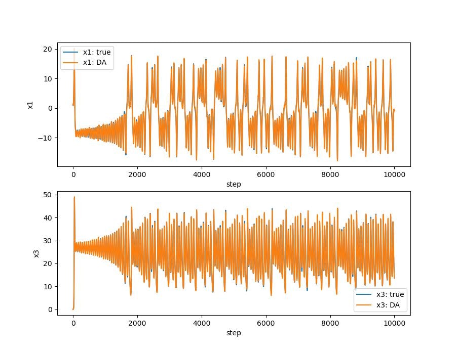
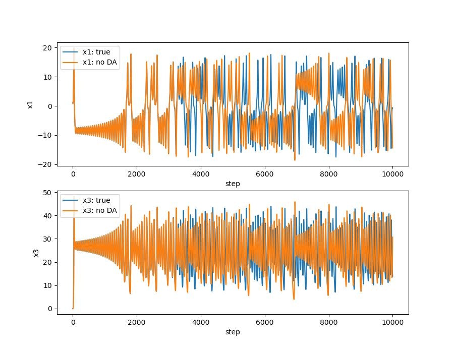
データ同化ありなしの比較

ローレンツ・アトラクタ。はじめのうちは3本とも重なっていますが，途中からずれてます。データ同化する（オレンジ）と真値とほぼ同様の解になります。

データ同化

Lorentz96の方は下記。

今回の数値解法は上記と同様，4次精度のルンゲ＝クッタです。

using PyPlot
using Random
using LinearAlgebra
using HDF5

function Lorentz63(x::Vector{Float64})
    σ::Float64 = 10
    ρ::Float64 = 28
    β::Float64 = 8/3
    
    Lorentz63 = zeros(3)
    Lorentz63[1] = σ*(x[2]-x[1])
    Lorentz63[2] = x[1]*(ρ - x[3]) - x[2]
    Lorentz63[3] = x[1]*x[2] - β*x[3]
    
    return Lorentz63
end

function RK4(f, dt, x)
    k1 = f(x)
    k2 = f(x + k1*dt*0.5)
    k3 = f(x + k2*dt*0.5)
    k4 = f(x + k3*dt)
    return x + dt*(k1 + 2k2 + 2k3 + k4)/6.
end

# 観測値の生成
function makeobs(y, xtrue, dstep, nmax)
    Random.seed!(10)
    for i=1:nmax
        if mod(i, dstep) == 0
            y[:,i] .= xtrue[:,i] .+ randn()
        end
    end
    
end

# Jacobianの生成
function makeM(x, N, dt)
    delta = 1e-2
    E = Matrix{Float64}(I, N, N)
    M = zeros(Float64, N, N)
    
    for j=1:N
        M[:, j] = (RK4(Lorentz63, dt, x + delta*E[:, j]) - RK4(Lorentz63, dt, x))/delta
    end
    
    return M
end

function main()
    nmax = 10000
    dstep = 5
    dt = 0.01
    
    x0 = zeros(3, nmax+1)
    x1 = zeros(3, nmax+1)
    x0[:,1] = [1.0, 0., 0.]
    x1[:,1] = [1.00001, 0., 0.]

    # x0が真値，x1が真値と初期値が若干異なる解
    for i=1:nmax
        x0[:, i+1] = RK4(Lorentz63, dt, x0[:,i])
        x1[:, i+1] = RK4(Lorentz63, dt, x1[:,i])
    end
    #println(x)
    
    y = zeros(3, nmax +1)     
    makeobs(y, x0, dstep, nmax)
    
    N = 3
    Xa = zeros(Float64, N, nmax+1)
    Xf = zeros(Float64, N, nmax+1)
    Pa = zeros(Float64, N, N, nmax+1)
    Pf = zeros(Float64, N, N, nmax+1)
    R = Matrix{Float64}(I, N, N)
    K = zeros(Float64, N, N)
    H = Matrix{Float64}(I, N, N)
    α = 1.5 # inflation factor
    
    println(Xa[:,1])
    
    Pa[:,:,1] = Matrix{Float64}(20I, N, N)
    
    Xa[:,1] = [1.00001, 0., 0.]
    println(Xa[:,1])
    
    for i=1:nmax
        Xf[:, i+1] = RK4(Lorentz63, dt, Xa[:,i])
        if mod(i+1, dstep) == 0
            M = makeM(Xf[:,i+1], N, dt)
            Pf[:,:,i+1] = α*M*Pa[:,:,i]*M'
            K = Pf[:,:,i+1]*H'*inv(H*Pf[:,:,i+1]*H' + R)
            Xa[:,i+1] = Xf[:,i+1] + K*(y[:,i+1]-H*Xf[:,i+1])
            Pa[:,:,i+1] = (I - K*H)*Pf[:,:,i+1]
        else
            Xa[:,i+1] = Xf[:,i+1]
            Pa[:,:, i+1] = Pa[:,:, i]
        end
    end

    # 結果の可視化
    plot_start=1
    plot_end=10000
    fig = plt.figure(figsize=(9, 7.))
    ax1 = fig.add_subplot(211)
    ax1.plot(x0[1,plot_start:plot_end], label="x1: true")
    ax1.plot(x1[1,plot_start:plot_end], label="x1: no DA")
    #ax1.plot(y[1,plot_start:plot_end], label="x1: obs.", "o", markersize=2.5)
    
    ax2 = fig.add_subplot(212)
    ax2.plot(x0[3,plot_start:plot_end], label="x3: true")
    ax2.plot(x1[3,plot_start:plot_end], label="x3: no DA")
    #ax2.plot(y[3,plot_start:plot_end], label="x3: obs.", "o", markersize=2.5)

    ax1.set_xlabel("step")
    ax1.set_ylabel("x1")
    ax1.legend()
    ax2.set_xlabel("step")
    ax2.set_ylabel("x3")
    ax2.legend()
    plt.savefig("true_noDA.jpeg")

    fig = plt.figure(figsize=(9, 7.))
    ax1 = fig.add_subplot(211)
    ax1.plot(x0[1,plot_start:plot_end], label="x1: true")
    ax1.plot(Xa[1,plot_start:plot_end], label="x1: DA",)
    #ax1.plot(y[1,plot_start:plot_end], label="u1", "o", markersize=2.5)
    
    ax2 = fig.add_subplot(212)
    ax2.plot(x0[3,plot_start:plot_end], label="x3: true")
    ax2.plot(Xa[3,plot_start:plot_end], label="x3: DA",)
    #ax2.plot(y[3,plot_start:plot_end], label="u3", "o", markersize=2.5)
    
    ax1.set_xlabel("step")
    ax1.set_ylabel("x1")
    ax1.legend()
    ax2.set_xlabel("step")
    ax2.set_ylabel("x3")
    ax2.legend()
    plt.savefig("true_DA.jpeg")
    
    rms_a = zeros(nmax+1)
    rms_o = zeros(nmax+1)
    trPa = zeros(nmax+1)
    for i=1:nmax
        trPa[i] = sqrt(tr(Pa[:,:,i])/N)
        rms_a[i] = norm(Xa[:,i]-x0[:,i])/sqrt(N)
        rms_o[i] = norm(y[:,i]-x0[:,i])/sqrt(N)
    end
    
    fig = plt.figure()
    ax1 = fig.add_subplot(111)
    ax1.set_ylim(-1,10)
    ax1.plot(rms_a[plot_start:plot_end], label="ana.")
    ax1.plot(rms_o[plot_start:plot_end], label="obs.", "o", markersize=2.5)
    ax1.plot(trPa[plot_start:plot_end], label="Trace")
    ax1.legend()
    
    ax = plt.figure().add_subplot(projection="3d")
    ax.plot(x0[1,plot_start:plot_end], x0[2,plot_start:plot_end], x0[3,plot_start:plot_end], )
    ax.plot(Xa[1,plot_start:plot_end], Xa[2,plot_start:plot_end], Xa[3,plot_start:plot_end], )
    #ax.plot(x1[1,100:300], x1[2,100:300], x1[3,100:300], )
    
    return x0, x1, Xa
end

実行と真値とデータ同化結果，データ同化なしの結果の出力

xtrue, x_noDA, Xa = main()

h5open("L63_true_da.h5", "w") do file
    write(file, "xtrue", xtrue)
    write(file, "Xa", Xa)
    write(file, "x_noDA", x_noDA)
end

ローレンツアトラクタの可視化

using Plots
using HDF5

file = h5open("L63_true_da.h5", "r") 
xtrue = read(file, "xtrue")
x_noDA = read(file, "x_noDA")
Xa = read(file, "Xa")

anim = @animate for i=2:100:9000
    plot(xtrue[1,i:i+300], xtrue[2,i:i+300],xtrue[3,i:i+300], label="true", 
        xlim = (-50, 50), ylim = (-50, 50), zlim = (0, 60),)
    plot!(Xa[1,i:i+300], Xa[2,i:i+300], Xa[3,i:i+300], label="DA", 
        xlim = (-50, 50), ylim = (-50, 50), zlim = (0, 60),)
    plot!(x_noDA[1,i:i+300], x_noDA[2,i:i+300], x_noDA[3,i:i+300], label="noDA", 
        xlim = (-50, 50), ylim = (-50, 50), zlim = (0, 60),)
    #plot!(sol2[1,i:i+300], sol2[2,i:i+300], sol2[3,i:i+300], 
    #    xlim = (-50, 50), ylim = (-50, 50), zlim = (0, 60), label="u0_2")
end

gif(anim, "lorentz3D-da.gif", fps = 2)

真値とデータ同化なしの解の比較。途中からずれてます。

真値とデータ同化後の解の比較