Python忘備録：Numpy配列の基本

はじめに

この記事は、英語の行列演算コースの内容を記録しているものです。もし間違っている箇所があれば、コメントでご指摘頂ければ幸いです。

少しデータサイエンスト向けにしています。

基本のキ

numpyをインポートします。

import numpy as np

np.array - 一次元配列

import numpy as np
a = np.array([1,2,3,4])
print(a)
# [1 2 3 4]

np.array - 二次元配列

import numpy as np
B = np.array([[0, 1, 2, 3],
              [4, 5, 6, 7],
              [8, 9, 10, 11]])
print(B)
# [[ 0  1  2  3]
# [ 4  5  6  7]
# [ 8  9 10 11]]

便利な array オブジェクトの属性

import numpy as np

C1 = [[0, 1, 2, 3],
      [4, 5, 6, 7],
      [8, 9, 10, 11]]

C2 = [[12, 13, 14, 15],
      [16, 17, 18, 19],
      [20, 21, 22, 23]]

C = np.array([C1, C2])

print(C.ndim) # 配列の次元数を表示　
print(C.shape) # 各次元の要素数。つまり、(ブロック数, 行数, 列数)
print(len (C)) # 配列の次元数を表示　
#3
#(2, 3, 4)
#2

Shape属性の特殊例 - 例えば(4,),(4,1),(1,4), (,4)

• 1次元配列：shape (4,)

import numpy as np

# 1次元配列：4個の要素を持つ
A = np.array([100, 200, 300, 400])
print("A =", A)           # 出力: [100 200 300 400]
print("A.shape =", A.shape)  # 出力: (4,)

• 2次元配列：shape (4, 1) (列ベクトル)

# 2次元配列：4行1列の列ベクトル
B = np.array([
    [100],
    [200],
    [300],
    [400]
])
print("B =\n", B)
print("B.shape =", B.shape)  # 出力: (4, 1)

• 2次元配列：shape (1, 4) (行ベクトル)

# 2次元配列：1行4列の行ベクトル
C = np.array([[100, 200, 300, 400]])
print("C =\n", C)
print("C.shape =", C.shape)  # 出力: (1, 4)

• (,4)は存在せず、(4,)となる

便利な Numpy 配列生成関数

import numpy as np
a = np.zeros((3, 3))
print(a)  # 3x3 のゼロ行列が出力されます。（NumPy配列）
#[[0. 0. 0.]
# [0. 0. 0.]
# [0. 0. 0.]]

import numpy as np
b = np.ones((3, 3))
print(b)  # 3x3 の1で埋められた行列が出力されます。（NumPy配列）
#[[1. 1. 1.]
# [1. 1. 1.]
# [1. 1. 1.]]

import numpy as np
c = np.eye(3)
print(c)  # 3x3 の単位行列が出力されます。単位行列（対角成分が1で、その他が0の行列）を生成します。
# Identity matrix
#[[1. 0. 0.]
# [0. 1. 0.]
# [0. 0. 1.]]
print(c.dtype) # floatで生成ｓれる
# float64

import numpy as np
vector = np.array([10, 20, 30])
diag_matrix = np.diag(vector)
print("対角行列:\n", diag_matrix)
# 出力:
# [[10  0  0]
#  [ 0 20  0]
#  [ 0  0 30]]
print(diag_matrix.dtype) # integerで生成される
# int64

# 例: 空の配列を生成
import numpy as np
empty_array = np.empty((3, 3))
print("初期化されていない配列:\n", empty_array)
# 出力例（実行するたびに異なる値が入ることがあります）:
# [[6.94699373e-310 0.00000000e+000 6.94699373e-310]
#  [6.94699373e-310 6.94699373e-310 6.94699373e-310]
#  [0.00000000e+000 6.94699373e-310 0.00000000e+000]]

# ランダムな数の配列を生成
import numpy as np
np.random.seed(3) # 乱数シードを設定
x=np.random.randint(0,20,15) # [0, 20) の範囲で 15 個の整数を生成
print(x)

配列スライス

• 基本スライシング

import numpy as np
a = np.array([0, 1, 2, 3, 4, 5])
print(a[1:5:2])  # 出力: [1 3]

• 多次元スライシング (Multidimensional Slicing)

import numpy as np
b = np.array([[0, 1, 2],
              [3, 4, 5],
              [6, 7, 8]])
print(b[0:2, 1:3])  # 出力: [[1 2]
                    #       [4 5]]

• ブールインデクシング (Boolean Indexing)

import numpy as np
x = np.array([-6, -3, 0, 3, 6, 9])
print(x[(x % 3 == 0) & (x > 0)])  # 出力: [3 6 9]

• 整数配列インデクシング (Integer Array Indexing)

import numpy as np
a = np.array([10, 20, 30, 40, 50])
indices = [0, 2, 4]
print(a[indices])  # 出力: [10 30 50]

• np.where を使った条件抽出

import numpy as np
x = np.array([1, 2, 3, 4, 5])
indices = np.where(x > 3)
print(indices)  # 出力: (array([3, 4]),)

• インデックスによるスライス

import numpy as np
np.random.seed(3)
x = np.random.randint(0, 20, 15) # 15 random ints in [0, 20)
print(x)
# [10  3  8  0 19 10 11  9 10  6  0 12  7 14 17]
inds = np.array([3, 7, 8, 12]) #配列から値を取り出すためのインデックス
print(x[inds]) #インデックスの番地にある値を表示
[ 0  9 10  7] # x[3] x[7] x[8] x[12]の値を表示している

• 奇数且つ０以上の値を表示するスライス

import numpy as np
x=np.random.randint(0,20,15)
result = x[(x% 3 == 0) & (x > 0)]
print(result)

乱数

Numpyには良い乱数生成関数が用意されています。
https://numpy.org/doc/stable/reference/random/index.html

from numpy.random import default_rng
rng = default_rng() # インスタンス rngを生成
A = rng.integers(-10, 10, size=(4, 3)) # -10以上10未満の整数を、形状(4,3)で生成
print(A)

平均、合計、最大、最小、標準偏差

import numpy as np
from numpy.random import default_rng
rng = default_rng()
A = rng.integers(-10, 10, size=(4, 3))
# 例
#[[  7,  -3,   1],
# [  3,   7,   2],
# [ -2,  -2,  -9],
# [ -9,  -6,   0]]
print(np.mean(A.T, axis=0)) 
# [ 1.66666667, 4.0, -4.33333333, -5.0 ]
# これは各Rowの平均を計算している
#　(7 + (-3) + 1) / 3 ≈ 1.67
# (3 + 7 + 2) / 3 = 4.0
# (-2 + (-2) + (-9)) / 3 ≈ -4.33
#  (-9 + (-6) + 0) / 3 = -5.0

print(np.mean(A.T))
# -0.9166666666666666
# A の全要素の平均（すなわち全体平均

print("np.max =", np.max(A, axis=1),"; np.amax =", np.amax(A)) #各行(横)最高値と全体の最高値
print("np.max =", np.max(A, axis=0),"; np.amax =", np.amax(A)) #各列(縦)の最高値と全体の最高値
# np.max() and np.amax() are synonyms
print("np.min =",np.min(A),"; np.amin =", np.amin(A))  # A 全体の中での最小値を返します
print("np.sum =",np.sum(A)) # A の全要素の和（合計）を計算
print("np.mean =",np.mean(A)) # A の全要素の算術平均（平均値）
print("np.std =",np.std(A)) # A の全要素の標準偏差（ばらつきの尺度）

絶対値

import numpy as np
from numpy.random import default_rng
rng = default_rng()
A = rng.integers(-10, 10, size=(4, 3))

print(A, "\n==>\n", np.abs(A))

#[[ 5 -9  1]
# [ 6 -3 -6]
# [-8  2  5]
# [ 2 -2  4]] 
#==>
# [[5 9 1]
# [6 3 6]
# [8 2 5]
# [2 2 4]]

既存の配列の形状情報を再利用

import numpy as np
from numpy.random import default_rng

A = np.array(
    [
        [5,-9,1],
        [6,-3,-6],
        [-8,2,5],
        [2,-2,4]
        ]
    )
A.shape # (4, 3)

rng = default_rng()
B = rng.integers(-10, 10, size=A.shape) #ここで再利用
print(B)
# [[ -1  -6   5]
# [  1   8  -4]
# [  2   8  -8]
# [ -1  -8 -10]]

２配列の各要素を比較し、大きい値を返す

#上記のコードの続き
C = np.maximum(A, B) # elementwise comparison
print(C)

ブロードキャスティング - Elementwise addition

A = np.array(
    [
        [5, -9, 1],
        [6, -3, -6],
        [-8, 2, 5],
        [2, -2, 4]
    ]
)
print(A)
#[[ 5, -9,  1],
# [ 6, -3, -6],
# [-8,  2,  5],
# [ 2, -2,  4]]

print(A + 3)
# [[ 8, -6,  4],
# [ 9,  0, -3],
# [-5,  5,  8],
# [ 5,  1,  7]]
 

データ点の重心-centroid（セントロイド）の計算

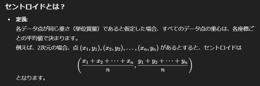
つまり、各列の平均値となる。従ってコードは以下となる

import numpy as np
# サンプルデータ点（例：2次元の座標）
points = np.array([
    [2, 3],
    [4, 1],
    [6, 7],
    [3, 5],
    [7, 3]
])

# セントロイド（各列の平均＝x座標の平均、y座標の平均）
centroid = np.mean(points, axis=0)
print(centroid) 
# [4.4 3.8]

# x 座標の平均は(2+4+6+3+7)/5=22/5=4.4
# y 座標の平均は(3+1+7+5+3)/5=19/5=3.8

センタロイドのシフト

import numpy as np

# 行列 A の定義（各行が1つのデータ点を表す）
A = np.array([
    [ 5, -9,  1],
    [ 6, -3, -6],
    [-8,  2,  5],
    [ 2, -2,  4]
])

# 各列の平均値（セントロイドの座標）を計算する
A_row_means = np.mean(A, axis=0) #　縦方向に計算！　
print("元の行列 A:")

print(A)
# 元の行列 A:
# [[ 5 -9  1]
#  [ 6 -3 -6]
#  [-8  2  5]
#  [ 2 -2  4]]

print("\n各列の平均 (セントロイド):")
print(A_row_means)

# 各列の平均 (セントロイド):
# [ 1.25 -3.    1.  ]

# ブロードキャスティングを利用して、各データ点からセントロイドを引く
# これにより、すべてのデータ点が平均 0 となるようにシフトされる
A_row_centered = A - A_row_means
print("\n中心化後のデータ (A_row_centered):")
print(A_row_centered)

# 中心化後のデータ (A_row_centered):
# [[ 3.75 -6.    0.  ]
#  [ 4.75  0.   -7.  ]
#  [-9.25  5.    4.  ]
#  [ 0.75  1.    3.  ]]

# 中心化後の各列の平均値を確認（ほぼ 0 になっているはずです）
print("\n中心化後の各列の平均:")
print(np.mean(A_row_centered, axis=0))

# 中心化後の各列の平均:
# [0. 0. 0.]

ブロードキャスティングの注意点

NumPy のブロードキャスティングは、配列の形状を右端から比較します。
各次元について、以下の条件のどちらかが満たされれば自動的に形状が合わせられます。

• 両方の次元のサイズが同じ
• どちらかの次元が 1

配列の形状の例

二次元配列。例：4 行 3 列の行列。

import numpy as np
A = np.arange(12).reshape(4, 3)
# A:
# [[ 0  1  2]
#  [ 3  4  5]
#  [ 6  7  8]
#  [ 9 10 11]]

• 一次元配列。例：4 個の要素を持つ

B = np.array([100, 200, 300, 400])
# B: [100 200 300 400]
# B.shape: (4,)

• 二次元配列（列ベクトル）。例：4 行 1 列

C = np.array([[100],
              [200],
              [300],
              [400]])
# C.shape: (4, 1)

• 二次元配列（行ベクトル）。例：1 行 4 列

D = np.array([[100, 200, 300, 400]])
# D.shape: (1, 4)

ブロードキャスティングが成功する場合の例

例: 配列 A の shape が (4,3) と、配列 B の shape が (4,1) の場合

• A の形状は (4,3)
• B の形状は (4,1) なので、B の右端の次元は 1です
• 右端の次元の1は、自動的に A の右端のサイズである3に拡張され、A と同じ形状 (4,3) となり、要素ごとの演算が可能になります

import numpy as np

A = np.arange(12).reshape(4, 3)
B = np.array([100, 200, 300, 400]).reshape(4, 1)
print("A + B =\n", A + B)

ブロードキャスティングが失敗する場合の例

例: 配列 A の shape が (4,3) と、配列 E の shape が (4,) の場合

• A の形状は (4,3)
• E の形状は (4,) ですが、ブロードキャスト時には自動的に (1,4) とみなされます
• 右端の次元で比較すると、A は 3、E（補完後）は 4となり、一致しないため演算ができずエラーになります

import numpy as np

A = np.arange(12).reshape(4, 3)
E = np.array([100, 200, 300, 400])  # shape: (4,)
# 以下はエラーになります:
# print(A + E)

(4,) の配列を (4,1) に変換すれば、ブロードキャストが正しく機能します。

E_fixed = E.reshape((4, 1))
print("A + E_fixed =\n", A + E_fixed)

Matrixの計算

1. 要素ごとの積（Hadamard 積）

要素ごとの積（Hadamard 積）とは、2つの同じ形状の行列や配列において、対応する位置の要素同士を掛け合わせる演算です。数式で表すと、行列 𝐴 と 𝐵のHadamard 積は以下のように定義されます。

$$(A∘B)_ij = A_ij \times Bij $$

特徴

• 要素ごとの演算: 通常の行列積（ドット積）は、行と列の内積を計算しますが、Hadamard 積は、各要素ごとに単純に掛け合わせます
• 形状の一致: 演算を行うためには、2つの行列または配列は同じ形状でなければなりません

import numpy as np

A = np.array([[1, 2],
              [3, 4]])
B = np.array([[5, 6],
              [7, 8]])

# 要素ごとの積（Hadamard 積）
C = A * B

print("A:\n", A)
print("B:\n", B)
print("Hadamard product (A * B):\n", C)

2. 行列積 Matrix Multiplication）

定義
2つの行列、たとえば

• 行列 A のサイズが m × k
• 行列 B のサイズが k × n

の場合、行列積（または行列の掛け算）は、サイズ m × n の新しい行列 C として定義されます。
各要素 $c_{i,j}$ は次のように計算されます。

$$ c_{i,j} = \sum_{s=0}^{k-1} a_{i,s} \times b_{s,j} $$

import numpy as np
from numpy.random import default_rng
rng = default_rng()

# 行列 A (サイズ: 4×3)
A = np.array([[  8,  -3,   3],
              [  7,   8,   0],
              [ -1,   9,   7],
              [ -8,  -7, -10]])
print(f"A ==\n{A}\n")

# 行列 B (サイズ: Aの列数×5 = 3×5)
B = rng.integers(-10, 10, size=(A.shape[1], 5))
print(f"B ==\n{B}")

# A ==
# [[  8  -3   3]
#  [  7   8   0]
#  [ -1   9   7]
#  [ -8  -7 -10]]

# B ==
# [[-2  8 -6 -2  8]
#  [-3  4 -7  0 -1]
#  [ 9 -1 -7 -3  0]]

# np.dot()
C = A.dot(B)
print(C)

# @ 演算子
C = A @ B
print(C)

#どちらとも以下になる
# [[  20   49  -48  -25   67]
#  [ -38   88  -98  -14   48]
#  [  38   21 -106  -19  -17]
# [ -53  -82  167   46  -57]]

終わりに

いかがでしたでしょうか？
何か誤記やご指摘ありましたら、コメントください。よろしくお願いします。

Happy Hacking!