Kaggle PlayGround 保険料の回帰予測 2024年12月

はじめに

毎月開催されている機械学習のシンプルな実践の場であるKaggle Play Ground。
こちらのコンペに参加をしたので、回帰分析の手順として当記事にまとめる。

KagglePlayGround遍歴(タイタニック除く)

シーズン	コンペ	KaggleScore	順位/参加数	上位%	1位Score
2024.4	アワビの 年齢当て	RMSLE: 0.14728	832/2608	31.9%	RMSLE: 0.14374
2024.7	自動車保険の 好意的反応	ROC-AUC: 0.89186	435/2236	19.4%	ROC-AUC: 0.89754
2024.8	キノコの 食用・有毒	MCC: 0.98488	472/2424	19.4%	MCC: 0.98514
🆕2024.12	保険料の 回帰予測	RMSLE: 1.04627	384/2390	16.1%	RMSLE: 1.01706

コンペ概要

• Kaggle Regression with an Insurance Dataset
• 期間：2024.12.01-12.31
• 参加期間：2024.12.04-12.31
• 目的：さまざまな要因に基づいて保険料を予測する。（回帰）
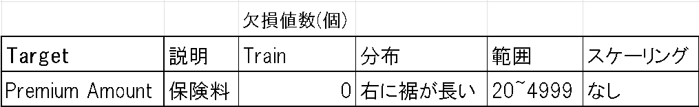
• ターゲット：'Premium Amount'
• 評価指標：RMSLE

評価指数：RMSLE

評価指数：RMSLE　
RMSLEは、予測値と実際の値との誤差を対数スケールで測定する指標。
特に金額や数量など, 範囲が広い場合に有効である。
対数スケールにより、数値が極端に小さい値や極端に大きな値を均等に評価できるためである。

• 対数変換
  • 実際の値と予測値を対数変換して計算
  • ⇒大きな予測誤差よりも小さな予測誤差を重視
  • ⇒これにより、極端な大きな値の影響を抑えられる
• 二乗誤差
  • 誤差を二乗して平均し、最終的に平方根を取る
  • ⇒誤差が大きいほどペナルティが大きくなる
• つまり
  • 極端な予測誤差を抑え、モデルが小さな誤差に過剰に反応するのを防げる

Ex. 理論上の話
✅例えばRMSLEが0だったとする。
⇒予測額と実際の保険額の間は対数スケールで0の誤差、つまり実測値と予測値が完全に一致していることを示す。
もし実際の保険額が100ドルであれば、予測額は100ドルである
👍値は0に近いほどモデルの性能が良いということになる。

実施環境・ライブラリ

●環境 : Google　Colaboratory

ライブラリ

# 基本のライブラリ
import pandas as pd
import matplotlib.pyplot as plt
import seaborn as sns
import numpy as np

# 前処理用
from sklearn.preprocessing import MinMaxScaler, StandardScaler, LabelEncoder

#特徴量選択用
from boruta import BorutaPy

# 学習モデル用
from sklearn.model_selection import train_test_split # データ分割
from sklearn.metrics import mean_squared_log_error # モデル評価RMSLE
import optuna # パラメータチューニング
from sklearn.model_selection import KFold #クロス交差検証用
from lightgbm import LGBMRegressor # LGBM
from xgboost import XGBRegressor # XGBoost
from catboost import CatBoostRegressor # CatBoost
from sklearn.ensemble import RandomForestRegressor # RandomForest
from sklearn.neural_network import MLPRegressor # MLP(ニューラルネットワーク)
from sklearn.ensemble import StackingRegressor # スタッキング用
from sklearn.linear_model import Ridge # リッジ回帰
from sklearn.linear_model import LinearRegression # 線形回帰

# 警告無視
import warnings
warnings.filterwarnings('ignore', category=UserWarning)

# 実行終了音
def beep():
  from google.colab import output
  output.eval_js('new Audio(\"https://upload.wikimedia.org/wikipedia/commons/0/05/Beep-09.ogg")\.play()')
#beep()

データの確認

Google Colabのファイルにデータセットをアップロード。

ディレクトリ

train.csv
test.csv

データの読み込み

df_train = pd.read_csv('train.csv')
df_test = pd.read_csv('test.csv')

データの表示（最初5行）

print('\n===df_train===\n')
display(df_train.head())
print('\n===df_test===\n')
display(df_test.head())

データの基本情報

print('\n==df_train info==\n')
display(df_train.info())
print('\n==df_test info==\n')
display(df_test.info())

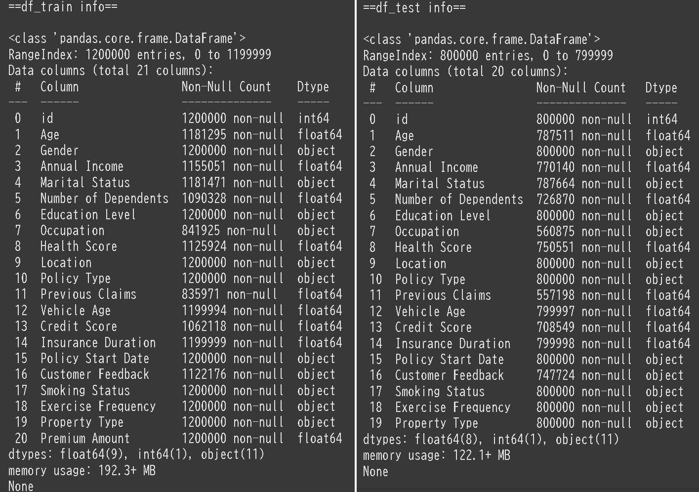
学習用データ：1200000行×21列
予測用データ：800000行×20列

基本統計量の取得

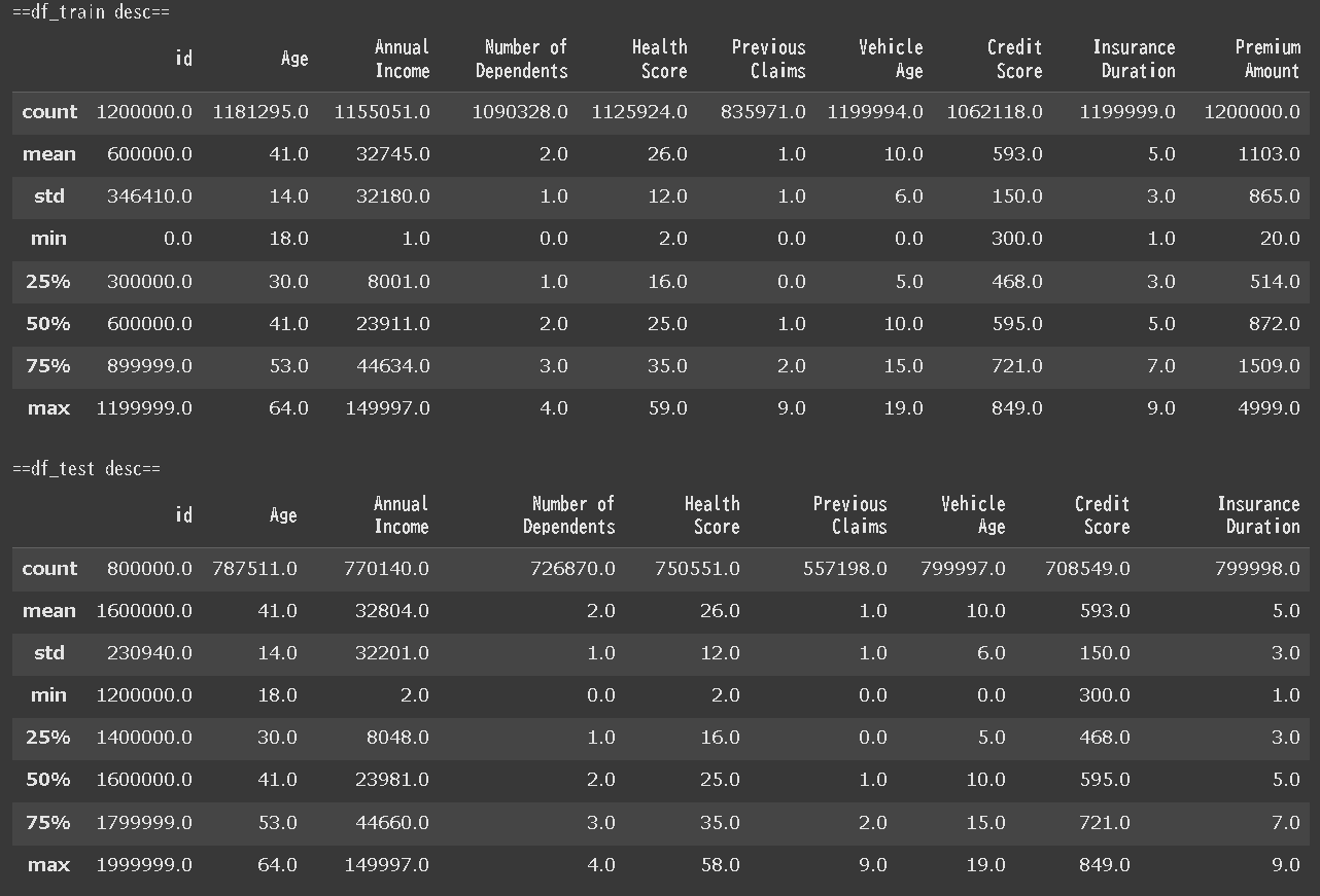
print('\n==df_train desc==')
display(df_train.describe().round())
print('\n==df_test desc==')
display(df_test.describe().round())

覚書一覧（折り畳み）

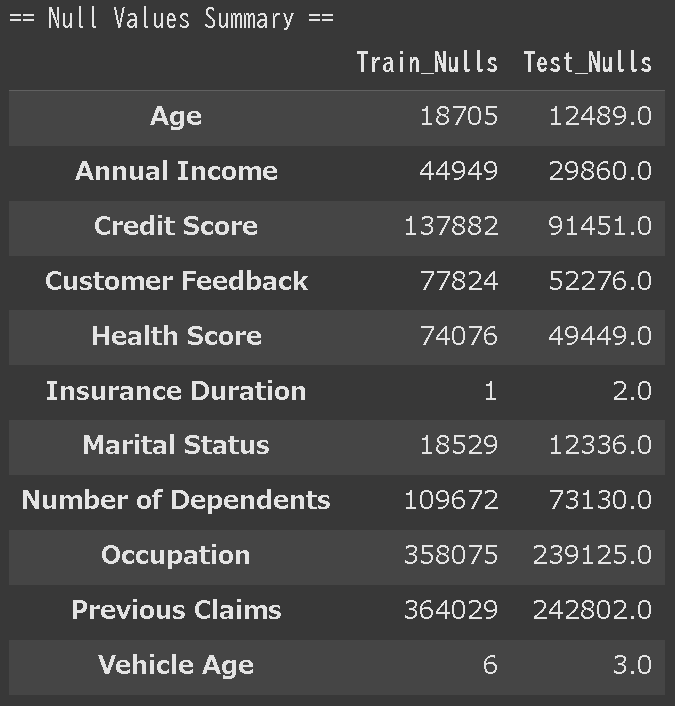
欠損値数だけ取得してデータフレームで見たいとき

# 欠損値のカウント
train_nulls = df_train.isnull().sum()
test_nulls = df_test.isnull().sum()

# データフレームにまとめる
df_null_summary = pd.DataFrame({
    'Train_Nulls': train_nulls,
    'Test_Nulls': test_nulls
})

# 欠損がある列のみを表示
null_summary_filtered = df_null_summary[(df_null_summary['Train_Nulls'] > 0) | (df_null_summary['Test_Nulls'] > 0)]

# 結果を表示
print("\n== Null Values Summary ==")
display(null_summary_filtered)

カラムだけ縦に並べて取得したいとき

print('\n'.join(df_train.columns))

ターゲット:Premium Amount(保険料)

量的変数

量的変数のグラフ(ヒストグラム)を確認したいときの関数

def con_chart(df_train, df_test, column_names):
    # 特徴量数に基づきサブプロット数を計算
    num_features = len(column_names)
    total_plots = num_features * 2  # 各特徴量でtrain/testのペア
    ncols = 2
    nrows = (total_plots + ncols - 1) // ncols  # 行数の計算（切り上げ）

    # グラフのサイズ調整
    fig, axes = plt.subplots(nrows, ncols, figsize=(10, 5 * nrows))
    axes = axes.flatten()  # 1次元配列に展開

    # 各特徴量でグラフを描画
    for i, column_name in enumerate(column_names):
        if column_name not in df_train.columns or column_name not in df_test.columns:
            print(f"Error: Column '{column_name}' does not exist in the DataFrame.")
            continue
        
        # df_train用のグラフ
        axes[i * 2].hist(df_train[column_name], color='skyblue', bins=30)
        axes[i * 2].set_title(f'df_train: {column_name}')
        axes[i * 2].set_xlabel(column_name)

        # df_test用のグラフ
        axes[i * 2 + 1].hist(df_test[column_name], color='lightgreen', bins=30)
        axes[i * 2 + 1].set_title(f'df_test: {column_name}')
        axes[i * 2 + 1].set_xlabel(column_name)

    # サブプロット間の余白調整
    fig.tight_layout()
    plt.show()

con_chart(df_train, df_test, ['Age', 'Annual Income', 'Number of Dependents', 'Health Score', 'Previous Claims', 'Vehicle Age', 'Credit Score', 'Insurance Duratio'])

質的変数

質的変数のグラフ(棒グラフ)を確認したいときの関数

def cat_chart(df_train, df_test, column_names):
    # 特徴量数に基づいてサブプロット数を計算
    num_features = len(column_names)
    total_plots = num_features * 2  # 各特徴量でtrain/testのペア
    ncols = 2
    nrows = (total_plots + ncols - 1) // ncols  # 行数の計算（切り上げ）

    # グラフのサイズ設定
    fig, axes = plt.subplots(nrows, ncols, figsize=(12, 5 * nrows))
    axes = axes.flatten()  # 1次元配列に展開

    for i, column_name in enumerate(column_names):
        if column_name not in df_train.columns or column_name not in df_test.columns:
            print(f"Error: Column '{column_name}' does not exist in the DataFrame.")
            continue

        # df_train用の棒グラフ
        category_counts_train = df_train[column_name].value_counts()
        category_counts_train.plot(kind='bar', ax=axes[i * 2], color='tomato', alpha=0.8)
        axes[i * 2].set_title(f'df_train: {column_name}')
        axes[i * 2].set_ylabel('Frequency')
        axes[i * 2].set_xlabel(column_name)

        # df_test用の棒グラフ
        category_counts_test = df_test[column_name].value_counts()
        category_counts_test.plot(kind='bar', ax=axes[i * 2 + 1], color='lightgreen', alpha=0.8)
        axes[i * 2 + 1].set_title(f'df_test: {column_name}')
        axes[i * 2 + 1].set_ylabel('Frequency')
        axes[i * 2 + 1].set_xlabel(column_name)

    # レイアウト調整
    fig.tight_layout()
    plt.show()

cat_chart(df_train, df_test, ['Gender', 'Marital Status', 'Education Level', 'Occupation', 'Location', 'Policy Type', 'Customer Feedback', 'Smoking Status', 'Exercise Frequency', 'Property Type'])

時間データ

契約開始日はobject型で格納されている。
Timedate型に変換し詳細を確認。時間はすべて同一であるため削除した。
分解・周期性各々に分けカラムを追加してみる。

df_1['Policy Start Date'] = pd.to_datetime(df_1['Policy Start Date'])

# 年、月、日、時間などを抽出
df_1['Start Year'] = df_1['Policy Start Date'].dt.year.astype('int16')
df_1['Start Month'] = df_1['Policy Start Date'].dt.month.astype('int8')
df_1['Start Day'] = df_1['Policy Start Date'].dt.day.astype('int8')

# 曜日（例: 月曜日=0, 日曜日=6）
df_1['Start Weekday'] = df_1['Policy Start Date'].dt.weekday.astype('int8')

# 年の何週目か
df_1['Start Week'] = df_1['Policy Start Date'].dt.isocalendar().week

#月の周期
df_1['month_sin'] = np.sin(2 * np.pi * df_1['Policy Start Date'].dt.month / 12)
df_1['month_cos'] = np.cos(2 * np.pi * df_1['Policy Start Date'].dt.month / 12)
#日の周期
df_1['day_sin'] = np.sin(2 * np.pi * df_1['Policy Start Date'].dt.day / 31)
df_1['day_cos'] = np.cos(2 * np.pi * df_1['Policy Start Date'].dt.day / 31)
# 曜日の周期性（0:月曜日〜6:日曜日）
df_1['weekday_sin'] = np.sin(2 * np.pi * df_1['Policy Start Date'].dt.weekday / 7)
df_1['weekday_cos'] = np.cos(2 * np.pi * df_1['Policy Start Date'].dt.weekday / 7)
# 季節の周期性（1年を4つの季節に分ける場合）
df_1['season'] = ((df_1['Policy Start Date'].dt.month % 12 + 3) // 3)
df_1['season_sin'] = np.sin(2 * np.pi * (df_1['Policy Start Date'].dt.month % 12) / 12)
df_1['season_cos'] = np.cos(2 * np.pi * (df_1['Policy Start Date'].dt.month % 12) / 12)

前処理・特徴量エンジニアリング

欠損値処理

試したこと
量的変数
・欠損値のある行を全削除
・単純補完(平均・最頻値・中央値)
・欠損値をそのまま維持
質的変数
・特定地('Unknown)で補完
・最頻値で補完
・欠損値をそのまま維持

結果
量的変数
・すべてを中央値で補完する

#量的変数　欠損値　削除  df_1['column'] = df_1['column'].fillna(df_1['column'].mean())
df_1['Age'] = df_1['Age'].fillna(df_1['Age'].median())
df_1['Annual Income'] = df_1['Annual Income'].fillna(df_1['Annual Income'].median())
df_1['Number of Dependents'] = df_1['Number of Dependents'].fillna(df_1['Number of Dependents'].median())
df_1['Health Score'] = df_1['Health Score'].fillna(df_1['Health Score'].median())
df_1['Previous Claims'] = df_1['Previous Claims'].fillna(df_1['Previous Claims'].median())
df_1['Vehicle Age'] = df_1['Vehicle Age'].fillna(df_1['Vehicle Age'].median())
df_1['Credit Score'] = df_1['Credit Score'].fillna(df_1['Credit Score'].median())
df_1['Insurance Duration'] = df_1['Insurance Duration'].fillna(df_1['Insurance Duration'].median())

質的変数
・特定値('Unknown)で補完

#質的変数　欠損値Unknown補完
df_1['Marital Status'] = df_1['Marital Status'].fillna('Unknown')
df_1['Occupation'] = df_1['Occupation'].fillna('Unknown')
df_1['Customer Feedback'] = df_1['Customer Feedback'].fillna('Unknown')

参考Kaggleノート : Relationship between NAN and Target

スケーリング・エンコーディング

試したこと
スケーリング
・標準化
・正規化
・対数変換
・スケーリングしない
エンコーディング
・ワンホットエンコーディング
・ラベルエンコーディング

結果
スケーリング

正規化

minmax_columns = ['Number of Dependents', 'Insurance Duration', 'Annual Income*Credit Score']

標準化

standard_columns = ['Health Score', 'Credit Score']

scaler = StandardScaler()
df_1[standard_columns] = scaler.fit_transform(df_1[standard_columns])

対数変換

log_columns = ['Annual Income', 'Previous Claims']

df_1[log_columns] = np.log1p(df_1[log_columns])

エンコーディング
・すべてをラベルエンコーディング

ラベルエンコーディング

# object型のカラムを取得
object_cols = df_1.select_dtypes(include=['object']).columns

# 各列をラベルエンコーディング
label_encoders = {}
for col in object_cols:
    le = LabelEncoder()
    df_1[col] = le.fit_transform(df_1[col])
    df_1[col] = df_1[col].astype('int8')  # int8型に変換
    label_encoders[col] = le

## 特徴量エンジニアリング
**ヒートマップ**
```Python:
# 数値データのみに限定
numeric_data = df_train.select_dtypes(include=['number'])

# ヒートマップの描画
plt.figure(figsize=(10, 8))
sns.heatmap(numeric_data.corr(), annot=True, cmap='coolwarm', fmt=".2f")
plt.title("Correlation Heatmap")
plt.show()

初期LGBMモデルで出した特徴量重要度

ヒートマップ・特徴量重要度からあたりをつけ、以下の特徴量を増産しつつ同一モデルで組み合わせや特徴量選択を繰り返す。

EX.

# 数値特徴量の組み合わせ df[''] = df[''] * df['']
df['Annual Income*Credit Score'] = df['Annual Income'] * df['Credit Score']

特徴量選択

ほとんどの特徴量のユニークな値は均衡なグラフを描いたことから、不要な特徴量として作用している可能性を考えた。収入と地域の組合せによる保険額の変化など探り学習してみる。
特徴選択のためのアルゴリズムBorutaを試してみたが、動作が上手くいかず手作業で試行。
特徴量重要度を確認しつつ、仮説検証を繰り返す。
最終的に以下の8つの特徴量に絞った。

'Premium Amount', 'Annual Income', 'Health Score', 'Credit Score', 
'Previous Claims','Start Year', 'Customer Feedback', 'Marital Status'

前処理・特徴量エンジニアリング最終コード

実施コード抜粋

# ======================================================================================
# データの結合
df_test['Premium Amount'] = 0
df = pd.concat([df_train, df_test], ignore_index=True)
# ======================================================================================

# -----------------------------------------------------------------------------------
# 時間データ
df['Policy Start Date'] = pd.to_datetime(df['Policy Start Date'])
df['Start Year'] = df['Policy Start Date'].dt.year.astype('int16')

# -----------------------------------------------------------------------------------
# 質的変数　欠損値Unknown補完
df['Marital Status'] = df['Marital Status'].fillna('Unknown')
df['Occupation'] = df['Occupation'].fillna('Unknown')
df['Customer Feedback'] = df['Customer Feedback'].fillna('Unknown')

# -----------------------------------------------------------------------------------
# 量的変数　欠損値　中央値補完
median_columns = [
    'Age', 'Annual Income', 'Number of Dependents', 
    'Health Score', 'Previous Claims', 'Vehicle Age', 
    'Credit Score', 'Insurance Duration'
]

df[median_columns] = df[median_columns].fillna(df[median_columns].median())

# -----------------------------------------------------------------------------------
# 数値特徴量の組み合わせ df[''] = df[''] * df['']
df['Annual Income*Credit Score'] = df['Annual Income'] * df['Credit Score']

# -----------------------------------------------------------------------------------
# 正規化
minmax_columns = ['Age', 'Number of Dependents', 'Vehicle Age', 'Insurance Duration']
scaler = MinMaxScaler()
df[minmax_columns] = scaler.fit_transform(df[minmax_columns])

# -----------------------------------------------------------------------------------
# 標準化
standard_columns = ['Health Score', 'Credit Score']
scaler = StandardScaler()
df[standard_columns] = scaler.fit_transform(df[standard_columns])

# -----------------------------------------------------------------------------------
# 対数変換
log_columns = ['Annual Income', 'Previous Claims']
df[log_columns] = np.log1p(df[log_columns])

# -----------------------------------------------------------------------------------
# ラベルエンコーディング
object_cols = df.select_dtypes(include=['object']).columns

label_encoders = {}
for col in object_cols:
    le = LabelEncoder()
    df[col] = le.fit_transform(df[col])
    df[col] = df[col].astype('int8')  # int8型に変換
    label_encoders[col] = le

# -----------------------------------------------------------------------------------
# 特徴量選択
df = df[['Premium Amount',
        'Annual Income', 'Health Score', 'Credit Score', 'Previous Claims',
        'Start Year', 'Customer Feedback', 'Marital Status', #'Annual Income*Credit Score']]

# ======================================================================================
# 結合解除
num_train_rows = len(df_train)
df_train_select = df.iloc[:num_train_rows].reset_index(drop=True)
df_test_select = df.iloc[num_train_rows:].reset_index(drop=True)
df_test_select = df_test_select.drop('Premium Amount',axis=1)

モデル構築・学習・評価

各モデルで特徴量選択を繰り返し、
手動であたりをつけた範囲からoptunaでのパラメータチューニングを実施。
以下でアンサンブルに使用した各モデルのパラメータを載せていく。
クロス交差検証を行ったものはRMSLEと平均値を記載している。

前処理にてスケーリングした際、負や0が出たためかエラー。
yを対数変換して対応。

説明変数X・目的変数yとデータの分割

X = df_train_select.drop('Premium Amount', axis=1)
y = df_train_select['Premium Amount']
X_train, X_test, y_train, y_test = train_test_split(X, y, test_size=0.2, random_state=42)

y_log = np.log1p(y) # 対数変換

X_train, X_test, y_train, y_test = train_test_split(X, y_log, test_size=0.2, random_state=42)

LightGBM

前処理・特徴量エンジニアリング等の基本モデルとして使用。

lgbm_params = {
    'boosting_type': 'gbdt',
    'objective': 'regression',
    'metric': 'l2',
    'n_estimators': 924, 
    'learning_rate': 0.015131582511543284, 
    'num_leaves': 77, 
    'max_depth': 33, 
    'min_data_in_leaf': 25, 
    'feature_fraction': 0.9911870244769206, 
    'bagging_fraction': 0.9088481641036802, 
    'bagging_freq': 2
}

lgbm = LGBMRegressor(**lgbm_params, random_state=42)

Fold 1 RMSLE for Fold 1: 1.0462945159070656
Fold 2 RMSLE for Fold 2: 1.0453838313527748
Fold 3 RMSLE for Fold 3: 1.0464000316055337
Fold 4 RMSLE for Fold 4: 1.0448637129856064
Fold 5 RMSLE for Fold 5: 1.0457226720021993

RMSLE CVMean: 1.04568
RMSLE CVSD: 

最初の半月はboosting_typeをabortで実行。
一番最初のSUBMITスコアは1.14235とベンチマークにも達していなかった。
abortからgbdtに変更し、ベンチマークを超えている。
パラメータの理解に課題が出た。

XGBoost

xgb_params = {
    'n_estimators': 1098,
    'learning_rate': 0.0201,
    'max_depth': 11,
    'subsample': 0.846,
    'colsample_bytree': 0.9,
    'gamma': 2.37,
    'reg_alpha': 2.76,
    'reg_lambda': 9.77
}

xgb = XGBRegressor(**xgb_params, random_state=42)

RMSLE: 1.04551

CatBoost

cat_params = {
    'iterations': 499, 
    'learning_rate': 0.07121886995402446, 
    'depth': 9, 'l2_leaf_reg': 4.539419279155112, 
    'random_strength': 0.2592634047515535, 
    'bagging_temperature': 0.12663365523881048, 
    'border_count': 237
}

cat = CatBoostRegressor(**cat_params, random_state=42)

Fold 1 RMSLE for Fold 1: 1.0467572161068095
Fold 2 RMSLE for Fold 2: 1.0461035194300858
Fold 3 RMSLE for Fold 3: 1.0469555238027097
Fold 4 RMSLE for Fold 4: 1.044610750663242
Fold 5 RMSLE for Fold 5: 1.0463931228671892

RMSLE CVMean: 1.04616
RMSLE CVSD: 0.00083

RandomForest

rf_params ={
    'n_estimators': 318, 
    'max_depth': 15, 
    'min_samples_split': 7, 
    'min_samples_leaf': 3}

rf = RandomForestRegressor(**rf_params, random_state=42)

RMSLE: 1.04581

MLP(ニューラルネットワーク)

MLP

mlp = MLPRegressor(
    early_stopping=True,
    hidden_layer_sizes=(25, 10),
    activation='relu',
    solver='adam',
    max_iter=500,
    random_state=42
)

RMSLE: 1.08227

アンサンブル学習

なるべくアルゴリズムの異なるモデルを組み合わせたい。

試したベースモデル

• 🚩LightGBM
• 🚩RandomForest
• 🚩CatBoost
• 🚩MLP
• XGBoost

試したメタモデル

• 🚩Ridge
• Liner

最終的に🚩のモデルの組合せがベストスコアとなった。

# ベースモデルの定義
base_models = [
    ("lgbm", LGBMRegressor(**lgbm_params, random_state=42)),
    ("randomforest", RandomForestRegressor(**rf_params_1, random_state=42)),
    ("catboost", CatBoostRegressor(**cat_params, random_state=42)),
    ('mlp', mlp)
#   ("xgboost", XGBRegressor(**xgb_params, random_state=42)),
]

# メタモデル
meta_model = Ridge(alpha=0.5, random_state=42)
# meta_model = LinearRegression(random_state=42)

# メタ特徴量を保存するための配列
meta_features = np.zeros((len(X_train), len(base_models)))

# ベースモデルのトレーニングと予測
for fold, (train_idx, val_idx) in enumerate(kf.split(X_train)):
    print(f"Fold {fold + 1}")
    X_fold_train, X_fold_val = X_train.iloc[train_idx], X_train.iloc[val_idx]
    y_fold_train, y_fold_val = y_train.iloc[train_idx], y_train.iloc[val_idx]
    
    for i, (name, model) in enumerate(base_models):
        model.fit(X_fold_train, y_fold_train)
        y_pred = model.predict(X_fold_val)
        
        meta_features[val_idx, i] = y_pred

# メタモデルのトレーニング
meta_model.fit(meta_features, y_train)

# テストデータのスタッキング
def predict_stacked(X_test):
    meta_test_features = np.zeros((len(X_test), len(base_models)))
    for i, (name, model) in enumerate(base_models):
        meta_test_features[:, i] = model.predict(X_test)
    return meta_model.predict(meta_test_features)

# テストデータでの予測
y_test_pred_log = predict_stacked(X_test)

# 元スケールに戻す
y_test_pred = np.expm1(y_test_pred_log)

# 評価
rmsle = np.sqrt(mean_squared_log_error(np.expm1(y_test), y_test_pred))
print(f'RMSLE: {rmsle}')

beep()

RMSLE: 1.0454153566307292

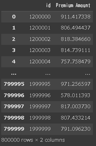
提出

予測データの予測

model_name = <モデルの名前を入力>

# モデルで予測
y_pred_log_test = model_name.predict(df_test_select)
# 予測値を逆変換（log1p の逆操作）expm1 で戻す
y_pred_test = np.expm1(y_pred_log_test)
# 提出用データの作成
df_submit = pd.DataFrame({
    'id': df_test_select['id'],  # テストデータのid列
    'Premium Amount':y_pred_test # 予測された保険額
})
df_submit

df_submit.to_csv('MODELNAME_00.csv', index=False)

コンペ最終結果

最終結果

順位は384/2390位（上位16.1%）
PRIVATEスコア　RMSLE:1.04627(1位スコア:1.01706)

PUBLIC
RMSLE: 1.04440
順位: 392位

PLIVATE
RMSLE: 1.04627 (+0.00187)
順位: 384位 (▲8)

過学習が起きていたか。
今コンペでは0.001単位での差が順位を大きく変えていた。
順位は上昇したが、他参加者のPUBLICとPLIVATEの差が大きかったことが影響していると思われる。

1位PUBLIC→PLIVATE：1.01587→1.01706
と同様の誤差あり。しかし1位の順位変動はなく、コンペ冒頭から他と大差をつけていた。
1.01台は1位のみである。

1位Kaggleノートブック : First Place - Single Model - [CV 1.016 LB 1.016]

やはりAutoMLか。

モデルの性能評価と解釈

LGBMモデルを例に性能評価と解釈を行う。

残差プロット

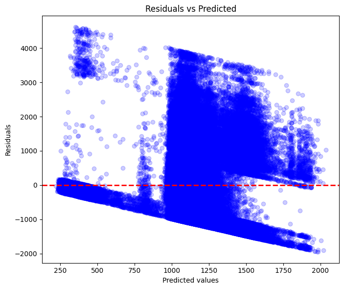
残差プロットが負の傾きを示している。
仮説
・モデルが過大予測している可能性
・モデルに非線形性が含まれる可能性
・重要な情報の欠落がある可能性

ヒストグラム　予測値VS実測値

仮説
・250～500の範囲で予測が嵌らない箇所がある。
　⇒除外すべき外れ値・異常値の存在がある可能性

（ここまででコンペ期限が迫り、検証をすっとばしてパラメータチューニングとアンサンブル学習に注力することとなった。）

まとめ

課題
・仮説検証といいつつ、場当たり的、総当たり的に行っている場面が多くみられた。機械的にグラフ化していくのではなく、データを読み取る前提を鍛えたい。
・各パラメータの値やアルゴリズムの理解が不足している。実施しているアルゴリズムがどういうもので、そのうえでどういった調整が必要なのか、何が読み取れるのか理解を深めていきたい。

感想
とはいえ前回より手順が円滑になり、順位・順位割合が向上。
まだまだ理解不足な部分が多いが、他人のコードの意味が分かるようになるなど成長も感じられた。
上位のコードは知らなかったり探索や分析の仕方で示唆が多い。
面倒くさがらずノートブック・ディスカッションをこまめにチェックするようにしていきたい。

今後のステップ
2025年1月現在、生存予測コンペが開催されている。
大変興味深いテーマであり、参加しようと思う。
競争率も高くより機械学習・統計の理解が必要であろうこちらを丁寧に実施したい。

参考URL

• 参加コンペデータ元： Regression with an Insurance Dataset
• Kaggle : 生存予測コンペ
• Qiita : RMSLEのはなし
• Kaggle : The Magic Middle - Median, Mean, or Exponented Mean Log 1p?
• Kaggle : Relationship between NAN and Target