緑本メモ: MCMCサンプルをJAGSとRで実行 - ランダム効果複数版 (10.5節) #R

緑本サイトからデータ d1.csv と階層ベイズのモデル定義 model.bug.txt (10.5節のもの) をダウンロードする。9章の例題をJAGSでやるメモの記載の通り、モデル定義にはJAGSで使えるように文末にセミコロンを足しておく。

下のようにしてパラメータの推定・事後分布の可視化と、MCMC収束診断の指数の出力をそれぞれ行う。

パラメータの推定と事後分布の可視化

下のRコードで、切片 $\beta_1$, 施肥処理の係数 $\beta_2$ , 個体差のばらつき $s$, 植木鉢効果のばらつき $s_p$ のパラメータ群をJAGSのMCMCによって推定する。

d <- read.csv("d1.csv")
filename <- 'model.bug.txt'

N.sample = nrow(d)
N.pot = length(levels(d$pot))

list.data <- list(
  N.sample = N.sample,
  N.pot = N.pot,
  N.tau = 2,
  Y = d$y,
  F = as.numeric(d$f == "T"),
  Pot = as.numeric(d$pot)
)

inits <- list(
  beta1  = c(0),
  beta2  = c(0),
  s     = c(1, 1),
  r     = rnorm(N.sample, 0, 0.1),
  rp    = rnorm(N.pot, 0, 0.1)
)

m <- jags.model(
  file = filename,
  data = list.data,
  inits = list(inits, inits, inits),
  n.chain = 3
)

update(m, 1000)

post.list <- coda.samples(
  m,
  c("beta1", "beta2", "s"),
  thin = 50, n.iter = 51000
)
summary(post.list)

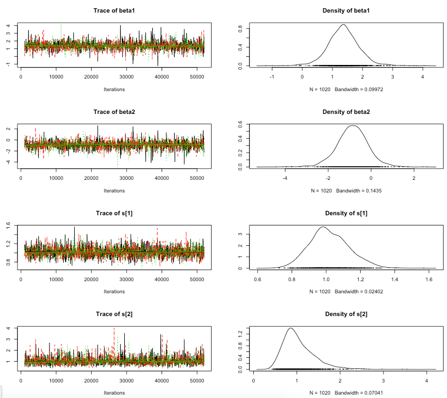
plot(post.list)

summary(..) で出力される各パラメータの推定値：

1. Empirical mean and standard deviation for each variable,
   plus standard error of the mean:

         Mean     SD Naive SE Time-series SE
beta1  1.3693 0.5279 0.009544       0.009732
beta2 -0.8736 0.7395 0.013368       0.013533
s[1]   1.0194 0.1153 0.002085       0.002084
s[2]   1.0453 0.3805 0.006879       0.006888

beta1, beta2 がそれぞれ $\beta_1$, $\beta_2$. s[1], s[2] がそれぞれ $s$, $s_p$.

plot(..) で出力される、サンプリングのトレース（左）と周辺事後分布の近似（右）の図：

MCMC収束診断

ランダム効果1個版と同様に R2jags で収束診断用の指数 $\hat{R}$ を出力する：

library('R2jags')
post.jags <- jags(
  data = list.data,
  inits = list(inits, inits, inits),
  parameters.to.save = c("beta1", "beta2", "s"),
  n.iter = 51000,
  model.file = filename,
  n.chains = 3,
  n.thin = 50,
  n.burnin = 1000)
print(post.jags)

出力結果（右から二番目の列に $\hat{R}$）：

Inference for Bugs model at "model.bug.txt", fit using jags,
 3 chains, each with 51000 iterations (first 1000 discarded), n.thin = 50
 n.sims = 3000 iterations saved
         mu.vect sd.vect    2.5%     25%     50%     75%   97.5%  Rhat n.eff
beta1      1.369   0.533   0.309   1.050   1.361   1.689   2.433 1.001  3000
beta2     -0.870   0.756  -2.375  -1.321  -0.855  -0.405   0.681 1.001  3000
s[1]       1.017   0.117   0.817   0.935   1.010   1.088   1.275 1.001  3000
s[2]       1.058   0.388   0.537   0.792   0.989   1.236   2.015 1.001  3000
deviance 367.798  13.090 344.504 358.482 366.919 376.521 394.577 1.001  3000

Rhat が1.0付近で1.1より小さければ収束していると判断。