はじめに
データ分析をやっていて、因果関係を知りたくなるのは世の常。特に複数の変数があって、それがお互いにどのように影響しているのか、ぱっと見ただけで分かるようなものはないのかと思って古典的ながらもベイジアンネットワーク分析をやってみました。
<環境>
Windows Subsystem for Linux、Ubuntu 18.04、R 3.6.2(Jupyter Notebook)
ベイジアンネットワークとは
こちらのページによると、”「原因」と「結果」の関係を複数組み合わせることにより、「原因」「結果」がお互いに影響を及ぼしながら発生する現象をネットワーク図と確率という形で可視化したものです。過去に発生した「原因」と「結果」の積み重ねを統計的に処理し、『望む「結果」に繋がる「原因」』や『ある「原因」から発生する「結果」』を、確率をもって予測する推論手法ともいえます。この考え方は人がさまざまな出来事や他人の振る舞いを予測するときの考え方に倣ったものといえます。”
ベイジアンネットワークをさくっとやるにはpythonよりもRの方がパッケージが充実しています。bnlearn、catnet、deal、pcalg、gRbase、gRainなどなど。今回は参考文献が充実しているbnlearnを使ってみました。
データ
今回はbnlearnの開発者が公開しているこちらのページにある"A Bayesian network analysis of malocclusion data"(不正咬合データのためのベイジアンネットワーク分析)の解析をなぞってみました。なお、私なりの解釈で一部のコードを変えているのはご了承ください。。
このデータは不正咬合の処置が上手くいくかを分析するためのデータになります。変数はそれぞれ以下のようになります(訳そうと思いましたが、専門用語が分からず…)。
- Treatment: untreated (NT), treated with bad results (TB), treated with good results (TG).
- Growth: a binary variable with values Good or Bad, determined on the basis of CoGn-CoA.
- ANB: angle between Down's points A and B (degrees).
- IMPA: incisor-mandibular plane angle (degrees).
- PPPM: palatal plane - mandibular plane angle (degrees).
- CoA: total maxillary length from condilion to Down's point A (mm).
- GoPg: length of mandibular body from gonion to pogonion (mm).
- CoGo: length of mandibular ramus from condilion to pogonion (mm).
str(ortho)

> 'data.frame':	143 obs. of  17 variables:
 $ ID       : Factor w/ 143 levels "P001","P002",..: 1 2 4 5 6 7 9 10 11 13 ...
 $ Treatment: Factor w/ 3 levels "NT","TB","TG": 1 1 1 1 1 1 1 1 3 1 ...
 $ Growth   : Factor w/ 2 levels "Bad","Good": 1 2 1 1 1 2 2 2 1 1 ...
 $ ANB      : num  -5.2 -1.7 -3.1 -1.3 0.4 1.5 -0.1 0.5 0.2 0.2 ...
 $ IMPA     : num  75.9 77.2 89.8 98.7 90.5 96.9 85.9 92 91.7 82.2 ...
 $ PPPM     : num  30.2 27 19.8 21.5 26.5 25.2 21.2 19.5 31.1 22.7 ...
 $ CoA      : num  83.4 91.3 78.6 96.4 83.3 88 85 77.1 88.8 77.5 ...
 $ GoPg     : num  77.9 84.1 67.3 75.6 74.7 72.8 75.2 65.2 76.2 67.8 ...
 $ CoGo     : num  50.1 59.2 50.4 65.7 51.3 58 54.9 44.8 53.3 44.5 ...
 $ ANB2     : num  -8.4 -2.3 -4.7 -2.4 -0.7 0.9 -1.3 0.4 0.8 -2.8 ...
 $ IMPA2    : num  71.7 81 83.8 86.6 83.8 95.8 87.7 93.6 92.3 82.6 ...
 $ PPPM2    : num  29.1 26.5 16.7 19.4 26.5 24.3 19.4 17.2 30.2 20.1 ...
 $ CoA2     : num  84.4 93.9 82.9 110.5 91 ...
 $ GoPg2    : num  81.9 84 71.5 96.3 83.5 71.8 76.9 69.3 81.3 82.5 ...
 $ CoGo2    : num  53.8 60.6 57.5 83.2 62.3 58.9 57.9 44.9 62 61 ...
 $ T1       : num  12 13 9 7 9 14 10 7 11 6 ...
 $ T2       : num  17 16 14 16 14 17 13 9 14 17 ...
今回の記事では時間を扱わない静的モデルでの分析を行いますので、少しデータを加工します。動的モデルは時間があれば書こうかな…。まずはT2時点とT1時点の差分を取っていきます。
diff = data.frame(
            dANB = ortho$ANB2 - ortho$ANB,
            dPPPM = ortho$PPPM2 - ortho$PPPM,
            dIMPA = ortho$IMPA2 - ortho$IMPA,
            dCoA = ortho$CoA2 - ortho$CoA,
            dGoPg = ortho$GoPg2 - ortho$GoPg,
            dCoGo = ortho$CoGo2 - ortho$CoGo,
            dT = ortho$T2 - ortho$T1,
            Growth = as.numeric(ortho$Growth) - 1,
            Treatment = as.numeric(ortho$Treatment != "NT")
)
Growthに関しては、生データが1と2だったので、1を引いて0と1に変換。Treatmentについては、Growthと一部、情報が被っているので、単に処置をしたかどうかのバイナリ変数にしています(NT=0, TBとTG=1)。
データ探索
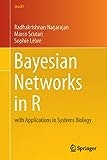
今回の変数は連続値を扱っていきますので、ベイジアンネットワークのモデル分類上はGaussian Bayesian Networksになります。Gaussianとついているように、データは正規分布に従っている必要があるほか、変数間が直線の関係を持つ必要があります。まずは正規分布の確認から。
par(mfrow = c(2,3), mar = c(4,2,2,2))
for(var in c("dANB", "dPPPM", "dIMPA", "dCoA", "dGoPg", "dCoGo")){
    x = diff[ ,var]
    hist(x, prob = TRUE, xlab = var, ylab = "", main = "", col = "ivory")
    lines(density(x), lwd = 2, col = "red")
    curve(dnorm(x, mean = mean(x), sd = sd(x)), from = min(x), to = max(x), add = TRUE, lwd = 2, col = "blue")
}
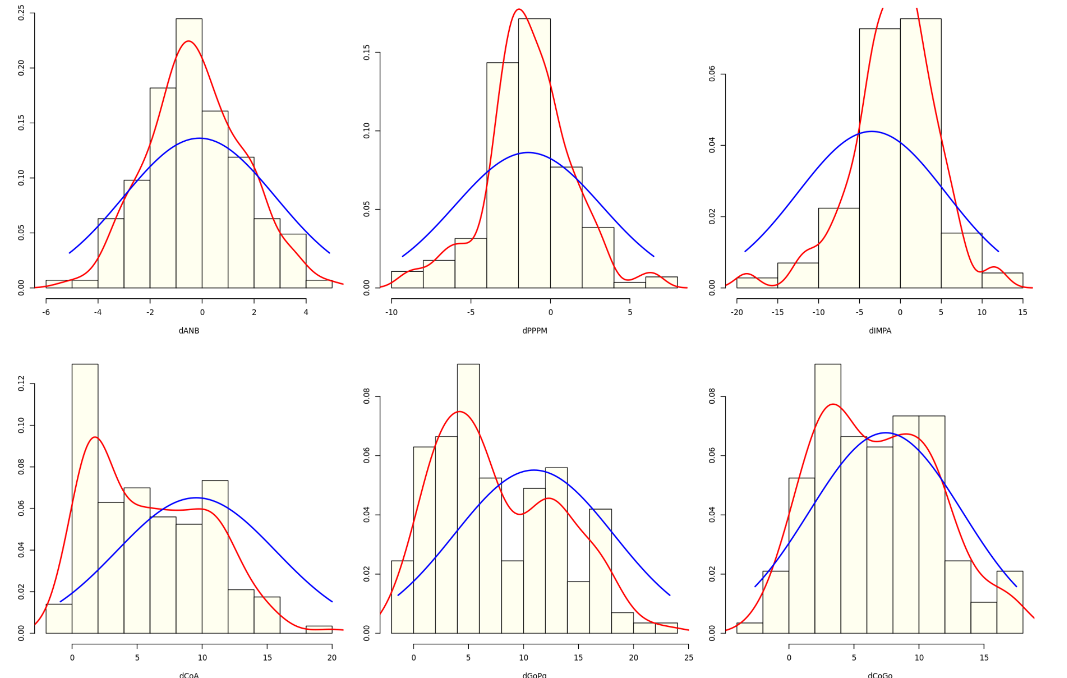
うーん、微妙。次に直線性の確認。
pairs(diff[, setdiff(names(diff), c("Growth", "Treatment"))],
     upper.panel = function(x, y, ...){
         points(x = x, y = y)
         abline(coef(lm(y ~ x)), col = "red", lwd = 2)
     },
     lower.panel = function(x, y, ...){
         par(usr = c(0,1,0,1))
         text(x = 0.5, y = 0.5, round(cor(x, y), 2), cex = 2)
     }
     )
こちらも一部はうまく当てはまっていますが、そうでないものも散見されます…。が、これについては、後程対処していきいます。
ネットワーク学習
ベイジアンネットワークの学習は2段階となります。まずは、どのようなネットワーク構造を持つのか(ネットワーク学習)、そしてそのネットワーク構造をもとにパラメータがどうなっているのか(パラメータ学習)です。まずは、ネットワーク学習から。これがとてつもなく難しい。
ネットワークの構造を特定するには、スコアベースアプローチと制約ベースアプローチという2つの大きなアプローが存在します。スコアベースアプローチの構造探索は、変数が増加すると指数関数的に計算量が増加する欠点が指摘されてきましたが制約ベースアプローチと比較して、サンプル数が少ない場合でも構造推定の精度を高く維持できるメリットがあります。ということで、今回はスコアベースアプローチを採っていきます。
スコアベースアプローチは次のようなネットワーク構造$G$のスコア関数が最大となる構造を探索するようなアプローチになります($X_i$は確率変数、$\Pi_{X_i}$はその確率変数の親)。
$$
Score(G) = \Sigma^N_{i=1} Score(X_i|\Pi_{X_i})
$$
スコアは対数尤度が多く使われてきましたが、過学習が問題となるため、BICやBDeなども開発されてきています。例えば、今回使用するBICであれば、以下のように罰則項が付け加えられます。
$$
BIC(G)=\Sigma^N_{i=1} logP(X_i|\Pi_{X_i}) - \frac{|\Theta_{X_i}|}{2} logn
$$
ということで構造学習の開始。まずはパッケージから。
library(bnlearn)
library(Rgraphviz)
bnlearnのほかにRgraphvizを読み込んでいます。これはグラフィカル分析を行う際に、グラフのプロットを綺麗にしてくれるもので、かなり良いです。現在はCRANに載っていないのでインストールする際はこちらの公式ページを参考にしてください。
ブラックリスト、ホワイトリスト
論理的に繋がってはいけないものをブラックリストとして指定できるほか、その逆をホワイトリストとして指定できます。ブラックリストとホワイトリストに指定する理由は元ページを確認ください。ここでは淡々と処理していきます。
bl = tiers2blacklist(list("dT", "Treatment", "Growth",
                         c("dANB", "dPPPM", "dIMPA", "dCoA", "dGoPg", "dCoGo")))
bl = rbind(bl, c("dT", "Treatment"), c("Treatment", "dT"))
bl

wl = matrix(c("dANB", "dIMPA",
              "dPPPM", "dIMPA",
              "dT", "Growth"),
         ncol = 2, byrow = TRUE, dimnames = list(NULL, c("from", "to")))
wl

構造学習
スコアベースアプローチでも色々なアルゴリズムが開発されていますが、ここではよくつかわれる山登り法(hill climbing)を用います。山登り法の説明はこちらを。計算途中が確認したければ、debug=TRUEとします。
dag = hc(diff, score = "bic-g", whitelist = wl, blacklist = bl)
dag

>  Bayesian network learned via Score-based methods
>
>  model:
>   [dT][Treatment][Growth|dT:Treatment][dANB|Growth:Treatment]
>   [dCoA|dANB:dT:Treatment][dGoPg|dANB:dCoA:dT:Growth]
>   [dCoGo|dANB:dCoA:dT:Growth][dPPPM|dCoGo][dIMPA|dANB:dPPPM:Treatment]
>  nodes:                                 9
>  arcs:                                  19
>    undirected arcs:                     0
>    directed arcs:                       19
>  average markov blanket size:           5.33
>  average neighbourhood size:            4.22
>  average branching factor:              2.11
>
>  learning algorithm:                    Hill-Climbing
>  score:                                 BIC (Gauss.)
>  penalization coefficient:              2.481422
>  tests used in the learning procedure:  157
>  optimized:                             TRUE
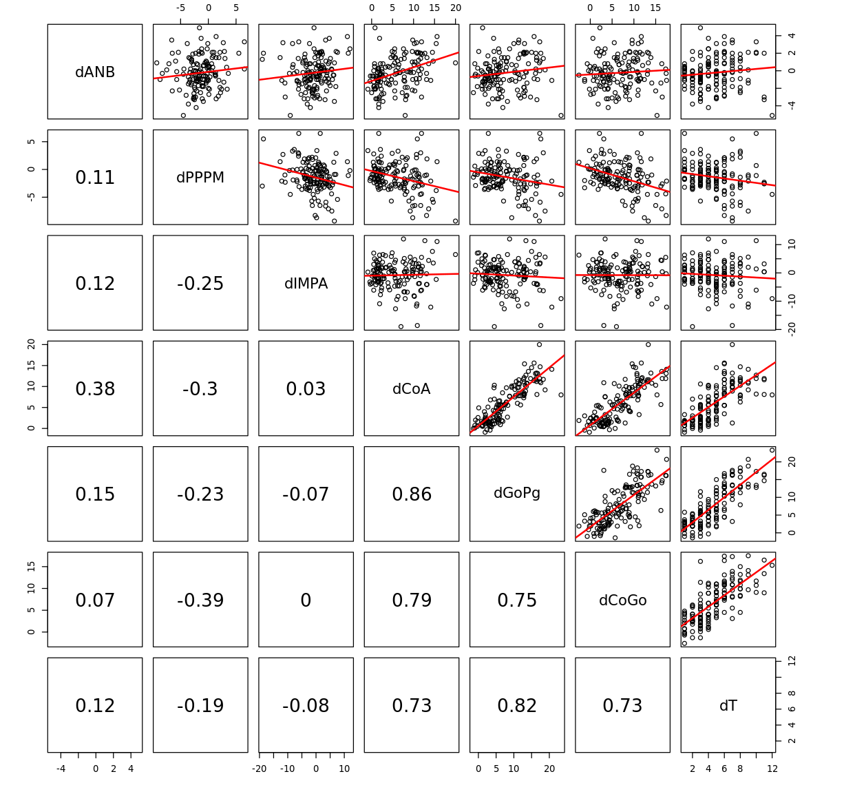
これをグラフで可視化すると、
graphviz.plot(dag, shape = "ellipse", highlight = list(arcs = wl))
ブートストラップ
しかしながら、このモデルは各変数が正規分布に従っているほか、変数間が線形で説明できるという仮定を満たしている必要があります。が、先ほどのデータ探索でそれが確認できなかったので、別のアプローチを行う必要があります。そこで、ブートストラップ法。boot.strengthで各変数間のつながりの強さと方向が確認できます。
str.diff = boot.strength(diff, R = 200, algorithm = "hc",
                         algorithm.args = list(score="bic-g",
                                               whitelist=wl,
                                               blacklist=bl))
head(str.diff)
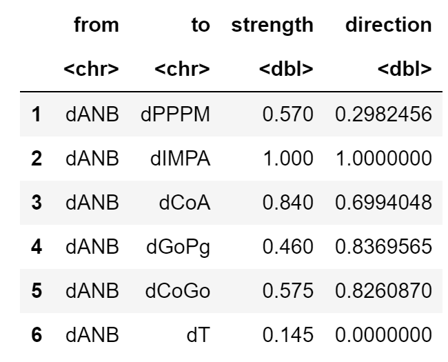
strengthは各変数のつながりの強さで最大値が1、directionは方向の強さで最大値は1になります。strengthが優位となる水準となる閾値は0.505となります。
attr(str.diff, "threshold")
> 0.505
plotで円弧の強さのCDFを確認できます。縦の点線が閾値になり、採用された円弧が点線の右側に存在するものになります。
plot(str.diff)

この閾値以上の強さを持つネットワークをaveraged.networkで取り出すことが出来ます。また、strength.plotで可視化できます。
avg.diff = averaged.network(str.diff)
strength.plot(avg.diff, str.diff, shape = "ellipse", highlight = list(arcs = wl))

ネットワークモデルの比較
graphviz.compareで2つの目で見て比較可能です。赤線が右のグラフのみにある円弧を、青線が左のグラフにのみある円弧を示しています。
par(mfrow = c(1,2))
graphviz.compare(avg.diff, dag, shape = "ellipse", main = c("averaged DAG", "single DAG"))

compareでも比較可能です。なお、arcs = TRUEとすると具体的な円弧が出てきます。
compare(avg.diff, dag)

> $tp
> 17
> $fp
> 2
> $fn
> 1
閾値の確認
先ほどCDFで閾値を確認しましたが、密度があまり高くない位置にありました。そこで、もう少し密度の高い値を探索します。
plot(str.diff)
abline(v = 0.75, col = "red", lty = 2, lwd = 2)
abline(v = 0.85, col = "blue", lty = 2, lwd = 2)

それぞれ採用される円弧の数は、
nrow(str.diff[str.diff$strength > attr(str.diff, "threshold") & str.diff$direction > 0.5, ])
nrow(str.diff[str.diff$strength > 0.75 & str.diff$direction > 0.5, ])
nrow(str.diff[str.diff$strength > 0.85 & str.diff$direction > 0.5, ])

> 19
> 15
> 12
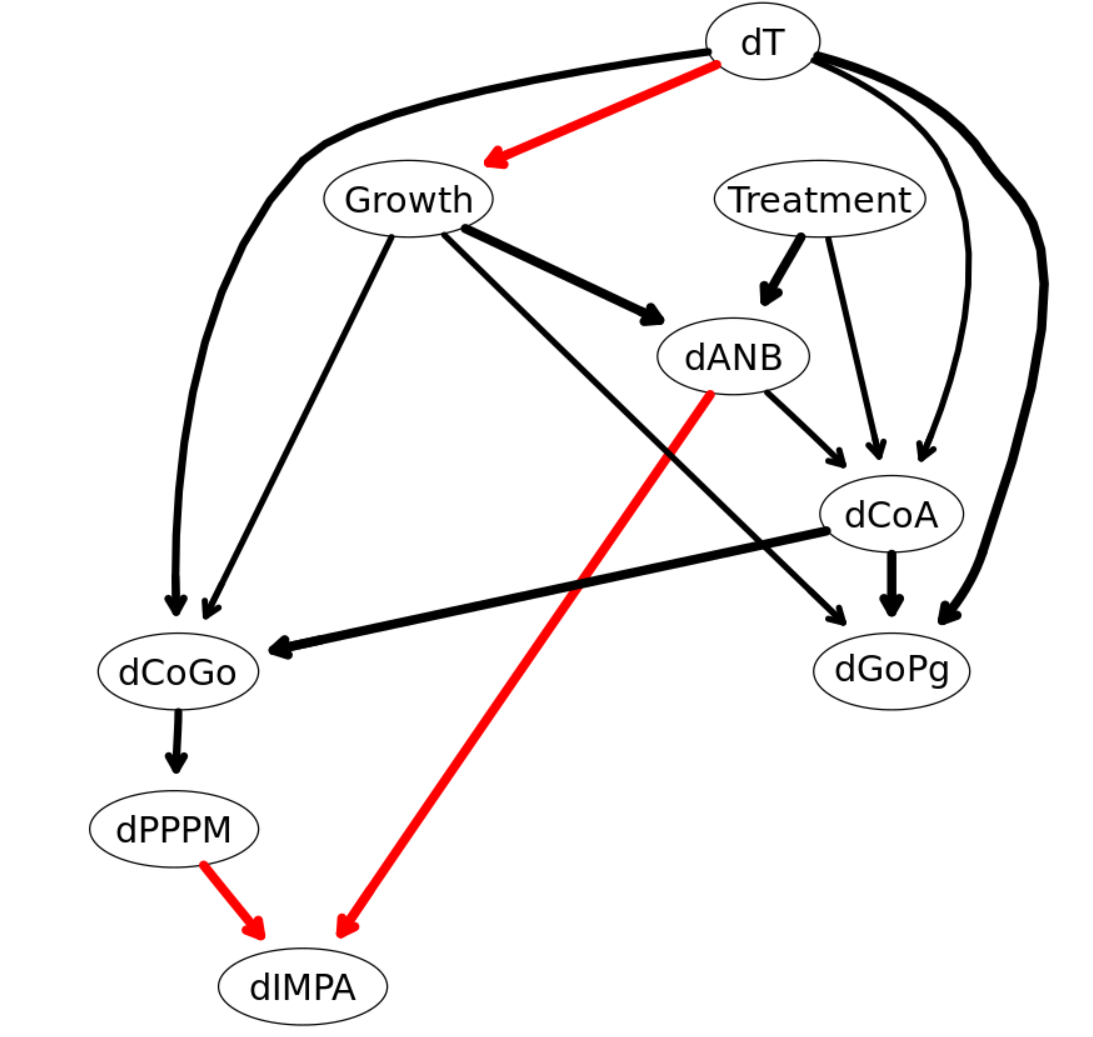
ということである程度の塊が確認できる0.75を採用。新しいネットワークモデルはこちら。
avg.simpler = averaged.network(str.diff, threshold = 0.75)
strength.plot(avg.simpler, str.diff, shape = "ellipse", highlight = list(arcs = wl))
ようやくネットワークのモデルが完成。
パラメータ学習
bn.fitでパラメータ学習ができます。ここでは、ネットワークモデルと、データを噛ませつつ、推定方法については、今回はガウシアンベイジアンネットワークになるので、最尤推定を用います。method = "bayes"でベイズ推定も出来ます。
fitted.simpler = bn.fit(avg.simpler, diff)
fitted.simpler

>   Bayesian network parameters
>
>   Parameters of node dANB (Gaussian distribution)
>
> Conditional density: dANB | Growth + Treatment
> Coefficients:
> (Intercept)       Growth    Treatment
>   -1.560045     1.173979     1.855994
> Standard deviation of the residuals: 1.416369
>
>   Parameters of node dPPPM (Gaussian distribution)
>
> Conditional density: dPPPM | dCoGo
> Coefficients:
> (Intercept)        dCoGo
>   0.1852132   -0.2317049
> Standard deviation of the residuals: 2.50641
>
>   Parameters of node dIMPA (Gaussian distribution)
>
> Conditional density: dIMPA | dANB + dPPPM
> Coefficients:
> (Intercept)         dANB        dPPPM
>  -1.3826102    0.4074842   -0.5018133
> Standard deviation of the residuals: 4.896511
>
>   Parameters of node dCoA (Gaussian distribution)

> Conditional density: dCoA | dANB + dT + Treatment
> Coefficients:
> (Intercept)         dANB           dT    Treatment
> -0.05370277   0.38905611   1.05794760   2.49280436
> Standard deviation of the residuals: 2.61764
>
>   Parameters of node dGoPg (Gaussian distribution)

> Conditional density: dGoPg | dCoA + dT + Growth
> Coefficients:
> (Intercept)         dCoA           dT       Growth
>   0.2065969    0.7149868    0.8334606   -1.6747242
> Standard deviation of the residuals: 2.233405
>
>   Parameters of node dCoGo (Gaussian distribution)
>
> Conditional density: dCoGo | dCoA + dT + Growth
> Coefficients:
> (Intercept)         dCoA           dT       Growth
>   1.5378012    0.5932982    0.5240202   -2.0302255
> Standard deviation of the residuals: 2.428629
>
>   Parameters of node dT (Gaussian distribution)
>
> Conditional density: dT
> Coefficients:
> (Intercept)
>    4.706294
> Standard deviation of the residuals: 2.550427
>
>   Parameters of node Growth (Gaussian distribution)
>
> Conditional density: Growth | dT
> Coefficients:
> (Intercept)           dT
>  0.48694013  -0.01728446
> Standard deviation of the residuals: 0.4924939
>
>   Parameters of node Treatment (Gaussian distribution)
>
> Conditional density: Treatment
> Coefficients:
> (Intercept)
>   0.4615385
> Standard deviation of the residuals: 0.5002708
>
それぞれのノードの関係は$で抽出可能です。
fitted.simpler$dANB

>   Parameters of node dANB (Gaussian distribution)
>
> Conditional density: dANB | Growth + Treatment
> Coefficients:
> (Intercept)       Growth    Treatment
>   -1.560045     1.173979     1.855994
> Standard deviation of the residuals: 1.416369
ちなみにこれは普通の回帰分析と同じ係数になります。
summary(lm(dANB ~ Growth + Treatment, data = diff))

> Call:
> lm(formula = dANB ~ Growth + Treatment, data = diff)
>
> Residuals:
>     Min      1Q  Median      3Q     Max
> -3.5400 -0.8139 -0.0959  0.7861  5.2861
>
> Coefficients:
>             Estimate Std. Error t value Pr(>|t|)
> (Intercept)  -1.5600     0.1812  -8.609 1.37e-14 ***
> Growth        1.1740     0.2440   4.812 3.82e-06 ***
> Treatment     1.8560     0.2403   7.724 1.96e-12 ***
> ---
> Signif. codes:  0 ‘***’ 0.001 ‘**’ 0.01 ‘*’ 0.05 ‘.’ 0.1 ‘ ’ 1
>
> Residual standard error: 1.416 on 140 degrees of freedom
> Multiple R-squared:  0.407,	Adjusted R-squared:  0.3985
> F-statistic: 48.04 on 2 and 140 DF,  p-value: < 2.2e-16
ここからgRainを使って詳細な分析ができるのですが、なぜかas.grainがうまく機能しないので、断念…。開発者が現在復旧作業しているというがいつになるのか…。
モデル評価
さて、最後はモデルの評価です。個々の円弧の関係を見ていく、推定されたパラメータを見ていくという方法のほかに、bnlearnではbn.cvで交差検証も可能です。まずはバイナリ変数のGrowthのCVを実行してから、そのほかの連続値の変数のCVを実行していきます。
xval = bn.cv(diff, bn = "hc", algorithm.args = list(blacklist=bl, whitelist=wl),
             loss = "cor-lw", loss.args = list(target = "Growth", n = 200), runs = 10)
err = numeric(10)
for(i in 1:10){
    tt = table(unlist(sapply(xval[[i]], "[[", "observed")),
               unlist(sapply(xval[[i]], "[[", "predicted"))>0.5)
    err[i] = (sum(tt) - sum(diag(tt))) / sum(tt)
}

summary(err)

>    Min. 1st Qu.  Median    Mean 3rd Qu.    Max.
>  0.2727  0.2797  0.2832  0.2867  0.2972  0.3077
predcor = structure(numeric(6), names = c("dCoGo", "dGoPg", "dIMPA", "dCoA", "dPPPM", "dANB"))
for(var in names(predcor)){
    xval = bn.cv(diff, bn = "hc", algorithm.args = list(blacklist=bl, whitelist=wl),
                 loss = "cor-lw", loss.args = list(target = var, n = 200), runs = 10)
    predcor[var] = mean(sapply(xval, function(x) attr(x, "mean")))
}


round(predcor, digits = 3)

> dCoGo0.849dGoPg0.905dIMPA0.224dCoA0.923dPPPM0.411dANB0.647

mean(predcor)

> 0.659720476350789
さいごに
と、長々と書き連ねてきましたが、データ探索からモデル評価までまとまった解説書(日本語、英語)がなかなか見つからなかったところ、開発者のHPにとてもいい事例があったので、勉強がてら参照させてもらいました。ところどころ、私なりの解釈でコードを変えているのはご了承ください。
記事にして分かることも多々あるので、時間があれば、山登り法に特有のスタート地点によっては局所的な最適解に陥ってしまう問題、時間を考慮した動的ベイジアンネットワーク分析なども記事にしていければと思っています。
参考文献